fbpx

Design of lattice girders based on EN 1993-1-1 standard

Software version:       ConSteel 17 Build 3303

Keywords:                  Modeling; Analysis; Design; Lattice girder; Getting started;

Model examples

Design objective, choice of design standard

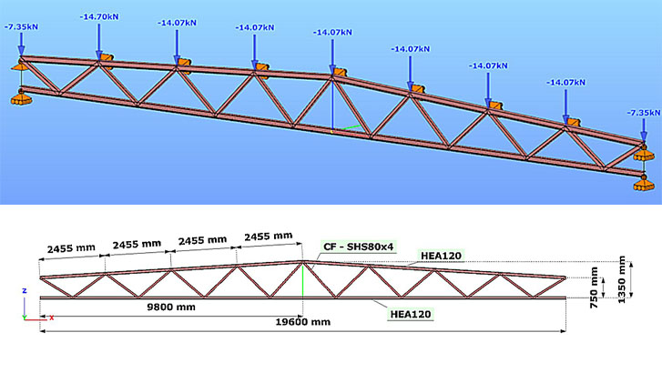
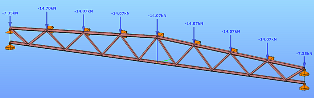
This design guide is intended for novice ConSteel 17 users and provides a step-by-step guide for designing a simply supported lattice girder. The geometry of the lattice girder to be designed is known from the architectural conceptual design, (Figure 1). According to the concept, the lattice girder chords are made of hot-rolled sections of HEA120, while the lattice bars  are made of cold-formed SHS80x4 sections. The design of the connections is not included in this guide.

Figure 1.  Geometric design of the lattice girder to be designed

(based on conceptual design)
Figure 1.  Geometric design of the lattice girder to be designed
(based on conceptual design)

It is well known that structural design is always carried out according to a certain standard or its version. The selection of the standard can be made from the Design Standard menu when creating a new model in the Project Center, or it can be modified later in the Standards tab [S1] selection panel (Figure 2).

Figure 2.  Choosing a design standard.
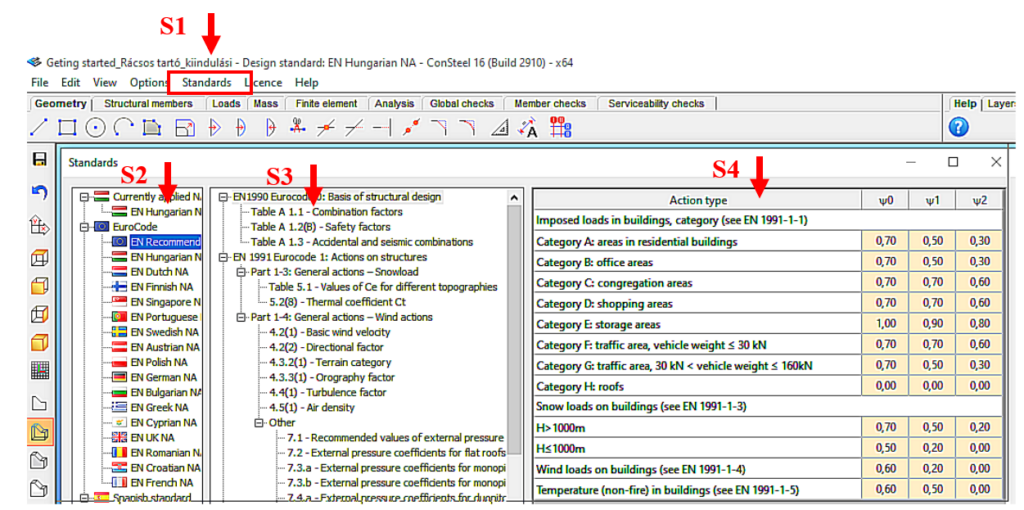
(S1: access standards; S2: select applicable standard; S3: select standard content; S4: display standard parameters).

The desired design standard can be selected from the list on the left of the panel. In this case, we select the EN Recommended option [S2]. The parameters applied by the selected standard can be accessed by selecting the corresponding row of the middle table [S3] of contents in the right-hand table [S4]. In Figure 2, the combination factors corresponding to Table 1.1 of the EC0 standard have been selected, whose parameters are shown in the right-hand table.

Setting the  grid raster editor

First, let’s set the size of the raster according to the span of the structure by using the corresponding button [1] of the tool group on the left, which will bring up the Grid and Coordinate System adjustment panel (Figure 3).

Figure 3.  Setting the editor raster
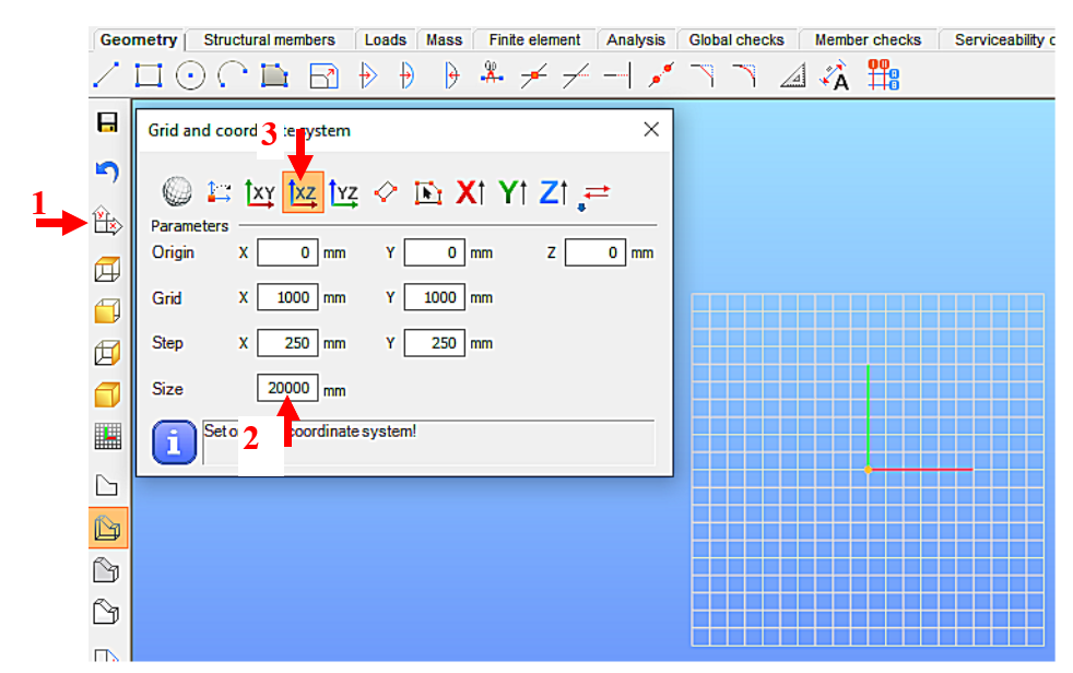
(1: set raster grid and coordinate system; 2: set raster occupancy size; 3: select view)

For example, for the 19.6m long support, the Size window can be set to 20000 millimeters [2]. To update the setting, press Enter. With the above setting, the raster will be 20m wide in X and Y directions, the raster line density will be 1000mm, and the step spacing will be 250mm. It is convenient to add the grid support model in the X-Z global coordinate plane, so the raster editor will be rotated to the X-Z plane. To do this, select the XZ plane option [3].

Loading initial cross-sections

One fundamental characteristic of general structural analysis programs is that they can only work with specifically defined cross-sections. Therefore, the first step is to choose the initial cross-sections for the task, according to the conceptual design. This may seem contradictory to the simple manual methods taught in basic statics courses, where the specific dimensions of the cross-section were often irrelevant information (e.g. calculation of internal forces). When using computer programs, however, we need to provide specific cross-sections even if their dimensions do not affect the static quantities to be calculated (e.g. in the present case, the normal forces of a truss beam). Nevertheless, we should aim to select cross-sections that match the geometrical size of the structure. In this case, the preliminary design served this purpose.

Initially, the section library for the current model is empty, so we first need to select the appropriate cross-sections. To do this, go to the Structure Members tab [4] and select the Section Administration option [5] on the left side of the horizontally positioned tool group, then select the "From Library..." button [6] in the panel that appears (Figure 4).

Figure 4.  Selecting the type of cross-section.
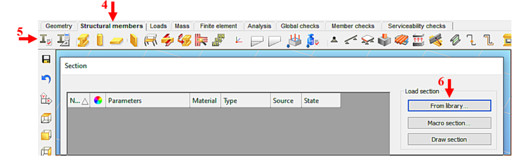
(4: picking up structural elements; 5: calling up the section control panel;
6: Select section type)

Figure 5 shows the loading of the HEA120 section, compliant with the European standard, which will be assigned to the chords. We select the region of the cross-section standard (European) and then its type (H profiles). From the list that appears, we can select the type of section (HEA) [7] and then the height of the section (120) [8]. By pressing the Load button [9], the program learns the cross-section, and from then on it knows everything about the cross-section and can work with it. Repeat the procedure as many times as you need different sections. Finally, the window is closed by pressing the Close button [10].

Figure 5. Selection of cross-section type and size (for European HEA120 profile).
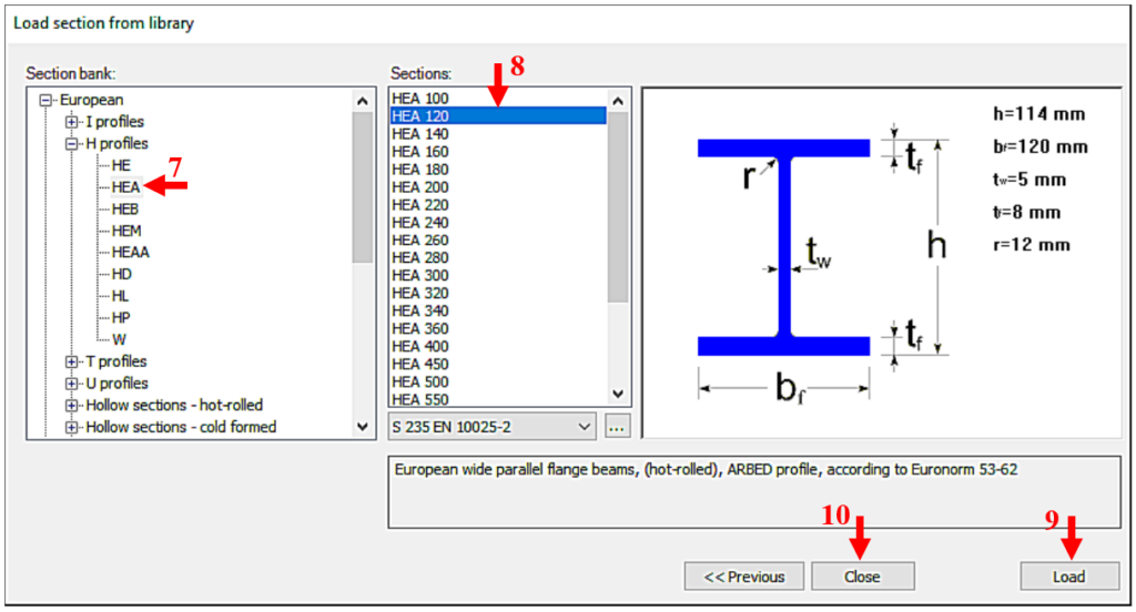
(7: select section type; 8: select section size; 9: scan selected section; 10: end loading process)

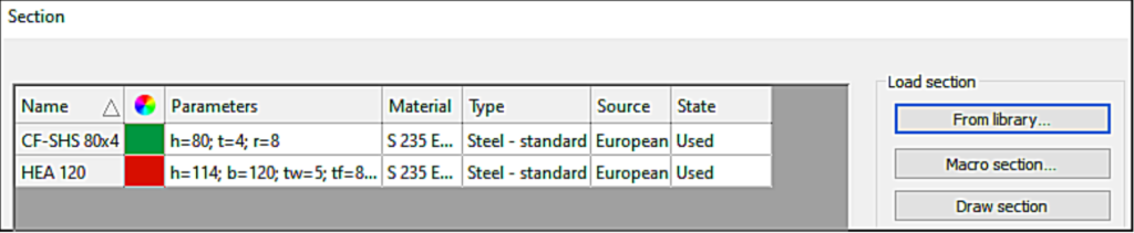
In our case, also a CF-SHS 80x4 closed section (from Library/Hollow sections - cold formed/CF-SHS/CF-SHS 80x4) was loaded for the bracing members (Figure 6).

Figure 6. Contents of the current cross-section store.

Later on, you can obtain all the information about the cross-section using the Section module. To do this, select the cross-section in the table by clicking on the corresponding row and then click on Properties... to display all the properties of the cross-section, such as type data; cross-section characteristics, etc. The program works with two cross-section mechanical models in a dual manner. The GSS (General Solid Section) model [11] is used for static calculations and the EPS (Elastic Plate Segment) model [12] for standard design operations (Figure 7). The cross-sectional properties (surface area, moments of inertia, etc.) can be displayed by pressing the button [13].

Figure 7.  Display of cross-sectional properties.
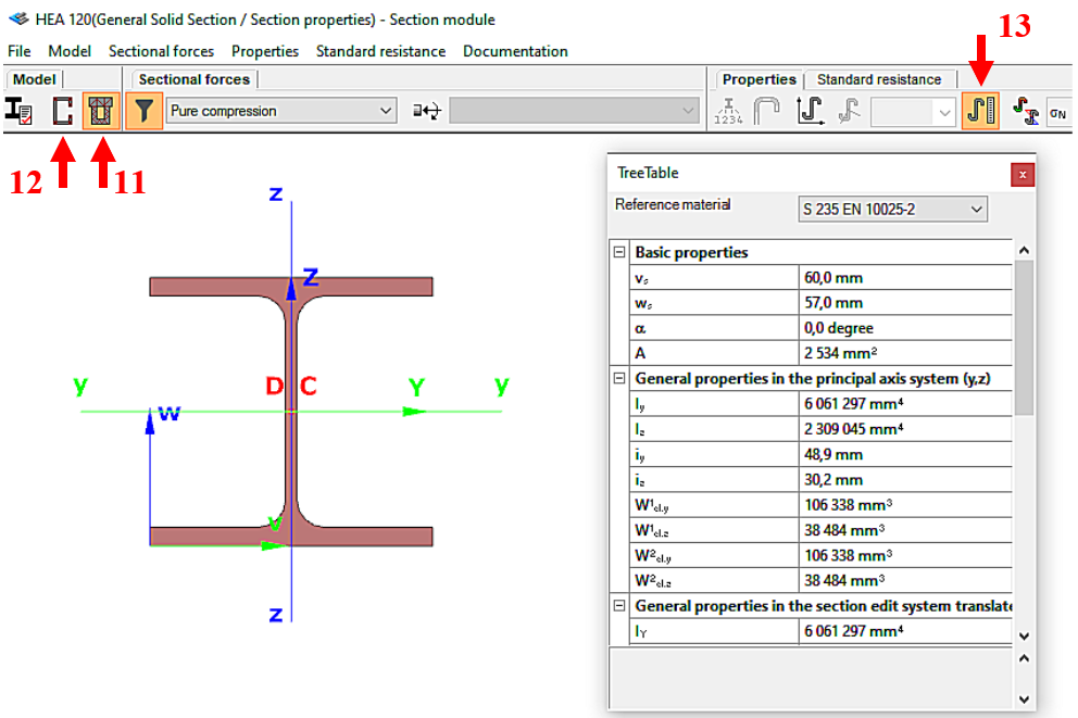
(11: Open GSS general section model; 12: Open EPS elastic plate segment model;
13: open cross-sectional properties table)

Building the structural model

Building of a structural (geometric) model consists of two main steps:

- creating the member geometry

- determining of supports.

Creating the member geometry

First, switch the coordinate input/display type to Absolute value setting. This is done using the switch [14] located in the bottom row of the editor window (if the Δ sign is yellow, the switch is set to Relative) (Figure 8).

Figure 8. Switch between Absolute/Relative coordinate values.
(14: Absolute/Relative coordinate value toggle button)

To begin creating the geometry, start by establishing the editing lines that define the structural shape. To do this, select the Draw Line function [15] under the Geometry tab (Figure 9).

Figure 9.  Drawing a line object.
(15: drawing lines; 16: drawing a section)

It's a good practice to establish the center of the lower chord of the truss at the origin of the global coordinate system, and from there, initiate the line segments using the drawing option [16]. The endpoints of these segments can be defined by specifying their X coordinate. The X (or any other) coordinate can be entered by typing the appropriate letter, entering the coordinate value in the corresponding coordinate window, and pressing ENTER. The result is shown in Figure 10. Of course, the network can be added in a different, possibly more practical order.

Figure 10.  The reference network of the lattice girder.

After creating the frame for the geometry, we proceed to add the bars that form the lattice girder. The frame serves as a good starting point for adding the bars, although it should be noted that one can also pick up the bars directly without the frame. The division of the chords into bars can be done in various ways: (i) each straight chord section consists of a single bar member, or (ii) both the upper and lower chords consist of two or more symmetrical bar members, or (iii) each section between nodes is a separate bar member. The choice will be determined by the design principle to be applied later: will the chord sections always consist of a single cross-section, or will the possibility of changing cross-sections within sections be retained? In the present case, we assume that we do not wish to change the cross-section along the chords, and therefore we prefer to choose solution (ii).

To add the members, we need to establish snapping points on the created reference lines. You can set the intercepts in the bottom right of the editor window. Since the bars are divided into eights along the lattice girder chords, we set n=8 [17] (Figure 11) and press Enter.

Figure 11.  Adjustment of the grip points (17: number of even divisions of the rod).

After the above adjustment, the red snapping points appear close to the reference line. You can create the bars by selecting two-two (start and end) snapping points (red dots) as follows. To add a bar, select the Edit Bar function [18] under the Structural Members tab. This will bring up the Member Editor dialog, where in this case it is sufficient to select the appropriate cross-section [19] (Figure 12).

Figure 12.  Preparing to place a structural member (bar).
(18: start member (beam) pick-up; 19: select cross-section)

The given bar can then be positioned using the snapping points. The operation is repeated until all the bars have been placed.

Based on the above steps, we create the structural model of the lattice girder: the lower and upper chords are modeled with two members (Figure 13), and the lattice members with a series of bar elements (Figure 14).

Figure 13. Model of chords of the structure.
Figure 14.  Series of bar members and the model of the complete lattice girder

The style of the model display can be selected using the style buttons in the left-hand column of the editor window (Figure 15).

Figure 15.  Selecting the display style of a structural model: (a) editor view; (b) wireframe view;
(c) backline view; (d) body view.

Adding supports

For general details about adding supports, see chapter 5.9 Supports in the Online Manual.  Here, only the support of the actual lattice girder is shown.

The grid of bars created in the previous section must be made structurally stable in 3D, i.e. properly supported. In the present case, we will add the following supports:

- XYZ fixed-pinned support at the top point on the left end of the truss;

- YZ-directional rolling-pinned support at the top point on the right-hand end of the truss;

- YZ-directional rolling-pinned supports at the end of the truss, in the nodes of the bottom chord.

- Y-directional pinned supports at the inner nodes of the upper chord.

As an example, place XYZ (spatial hinge) support at the top left end node of the truss. Select the Point Support function [20] under the Structural Members tab, which will display the adjustment dialog (Figure 16). The support type can be selected in the upper window of the dialog [21].

Figure 16.  Positioning of a point support.
(20: point support placement; 21: point support type selection)

For the graphical display of the point supports, we recommend the hidden line or solid view (Figure 16. c or 16.d). It is possible that the graphical symbol of the placed support may not be visible due to its relatively small size and/or being obscured. It is a common mistake that the user does not see the placed support and places it multiple times on the same node: this will result in a model error later! The size of the graphic symbol can be increased by using the adjustment slider at the bottom right of the editor window [22] (Figure 17). Use the slider or, if necessary, the arrow to increase the size of the graphic symbol of the support object until it is sufficiently visible. If the support is obscured, it becomes visible by rotating the model.

Figure 17.  Setting the dimensions of graphic objects.
(22: support graphic object size adjustment)

You can place the supports one after the other, using the left mouse button, at the corresponding nodes of the model. The complete support system, and thus the complete structural model, is shown in Figure 18.

Figure 18.  The support system and the complete structural model.

Load model creation

Load model structure

First, let's determine the structure of the load model. Select the Load Cases and Load Groups function [23] under the Load tab, which will bring up a panel defining load groups and load cases (load case = a group of loads that are inseparable in time and space; load group = a group of load cases where the loads can be mutually exclusive in load combinations) (Figure 19). When a new model is created, the load structure on the left side of the dialog box contains by default one load group with one load case.  Start by selecting the appropriate load group or load case name on the left, then rename it on the right to a name that suits your needs.

 For example, change the initial name of the load group to 'Dead load' [24] and the name of the load set to 'Self-weight' [25]. Confirm the action with the Apply button.

Figure 19.  Load group and load case renaming.
(23: Manage load cases and load groups; 24: Enter load group name; 25: Enter load case name)

If you have more than one load case in the ’Dead Load’ load group, you can add them [27] by using the New load case button [26] in the bottom table of the dialog (Figure 20).

Figure 20.  Adding a new load case within a given load group.
(26: add a new load case; 27: enter the name of the new load case)

You can add a new load group by clicking on the New load group button [28] at the top of the dialog, but first select the appropriate category in the window [29] next to it. In this case, the new load group contains snow, so select the ’Snow’ option (Figure 21).

Figure 21.  Adding a new load group.

Based on the well-thought-out load model, all load groups and load cases are added by repeating the above operations (Figure 22).

Figure 22.  Load model structure.

As a final step, assign the automatically generated structural self-weight to a selected load case. To do this, open the drop-down list Load case including self-weight [30] at the bottom of the table and select the appropriate load case, in this case the load ‘Self-weight’ (Figure 23). Finally, close the window by clicking on OK. This defines the structure of the load model. In the next step, we will apply loads to the appropriate load cases.

Figure 23.  Assigning the structural dead load to a load case, in our case to the 'Self-weight' load case.
(30: selecting a load case for the self-weight load)

Loading load cases

We start to add actual loads to the load cases recorded in the load model structure. This can be a lengthy process, so we will first summarise the most important technical elements of applying loads and then present the actual loads.

Technical elements

Let us open the window under the Loads tab [31], where we select the load case to which we will assign specific load components (Figure 24).

Figure 24.  Selecting the load case (31: open a drop-down list and select the load case to be uploaded)

The loads added next are added to this load case until the selection above is overwritten by another selection. We will now describe the elements and technical aspects of load application. In the case of lattice girders, the loads are usually concentrated forces (the bars of a lattice girder are usually not directly loaded). Therefore, only the definition of the concentrated force is discussed below.

Concentrated load in the global system

Select the Point Load function [32] under the Loads tab, and then enter the components of the concentrated force as interpreted in the global system [33] in the corresponding input fields [34]. Clicking on the corresponding structural node will place the concentrated force in the structural model as part of the current load case (Figure 25).

Figure 25.  Plot of concentrated force at structural nodes.
(32: start concentrated load placement; 33: select global system;
34: specify concentrated load components)

Concentrated load in the local system

In certain types of loads, the direction of the concentrated force may not align with the direction of the global coordinate system. For example, in the case of wind loads, the load may act perpendicular to the roof surface, in our case the upper chord. In such cases, instead of calculating components in the global directions, we switch to the local system. To do this, we select the Local coordinate system option [35], after which the concentrated load [36] can be placed on the structural model in two steps: (1) selecting the appropriate structural node with the mouse, and then (2) selecting the relevant member whose axis forms the X coordinate axis of the local system (Figure 26).

Figure 26.  Placement of concentrated force at structural nodes in the local system,
 in our case perpendicular to the axis of the chord.
(35: switch to the local system; 36: specify load components; (1) click to node; (2) click to member)

Applied load cases

Using the above technical elements, the following load cases have been applied:

Load combinations

The next step is to create load combinations. To do this, select the Load Combinations button [37] under the Loads tab, which will bring up the Load Combinations table. Select the option "Automatic generation of load combinations" [38], which will display the symbolic formulas of the load combination types for the design situations (Figure 27).

Figure 27.  Automatic generation of load combinations, and selection of design situation(s).
(37: start definition of load combinations; 38: automatic generation of load combinations)

In our case, we need the options 'Persistent and transient design situations - Eq. 6.10' and 'Accidental design situation - Eq. 6.11.b'. The setting is confirmed with the Apply button, which causes the generated load combinations to appear in the table (Figure 28). In the table, if necessary, undesirable combinations can be deleted after selection [39], partial factors can be rewritten, and new combinations can be created if necessary [40].

Figure 28.  Table of automatically generated load combinations.
(39: delete combination row(s); 40: add new combination row)

Verifying the structural model

Before performing a final analysis, it is useful to ensure that the structural model is correct. Select the Analysis Parameters button [41] under the Analysis tab, which will bring up the analysis setup dialog, where you should first select only the "First order analysis" option [42] (Figure 29).

Figure 29.  Setting the analysis type.
(41: call up the analysis setup panel; 42: select the first order analysis; 43: possibility to set the detailed setup)

Switch to the load combinations table [43] and switch off all combinations (select all the checkboxes in the Load combination set field with a left-click, then right-click on any checkbox to clear the checkmarks), except one in which only symmetric loads are present (in our case, this is load combination 3 (Lc-3), in which only the permanent load and the total snow load are present) (Figure 30).

Figure 30.  Selection of a symmetric load combination for structural model checking.

After the setup, press the Apply and Calculate buttons, wait for the analysis to run, and then examine the results. Possible aspects of the analysis are summarised below.

After the analysis is performed, the deformed shape of the structure is displayed. The deformation diagram can be scaled by using the slider next to the adjustments fields [44]. The content of the graphical display can be adjusted by using four fields (Figure 31). The contents of the windows are as follows:

- selection of analysis types (first-order; second-order; stability; etc.) [45];

- selection of load combination or load set [46];

- selection of the type of data to be displayed (displacements; stresses; etc.) [47];

- select the type of drawing (diagram; color overlay; etc.) [48].

Figure 31: Display of the deformed structural shape and scaling of the figure.

Let's examine the displayed deformed shape. Aspects of the test are usually the following:

  • Is the deformed shape symmetric for symmetric loads...?
  • Does the deformed shape stay within the plane of the model for loads in the plane...?
  • Is the maximum displacement value realistic...?
  • Does the deformed shape adhere to engineering judgment...!?

In the next step, let us switch to the internal forces, in our case the "N" normal force plot [49] (Figure 32), and examine the plot from the following points of view:

  • Does the axial force decrease in the top chords of the trusses toward the ends of the beams...?;
  • Is the value of the maximum normal force in the chords realistic...?;
  • Does the axial force decrease in the diagonal bracing towards the center of the beam...?;
  • Does the shape of the diagram adhere to engineering judgment (e.g., are there tensioned bars along the top chord of a two-span beam or compressed bars along the bottom chord)...!?
Figure 32. Choosing the type of demand internal force.
(49: select the internal force to be displayed)

Analysis 

If the result of the model check in the previous step is successful, we can proceed to the final analysis. To do this, enable all relevant load combinations and then perform the first-order analysis. If the calculation finishes without an error message, the model is ready for design.

The first step is to determine the relevant load combination (perhaps the first two or three) for which you want to save the figures and use them in other documents. This is done by using the automatic cross-section check function of the program (Figure 33). Switch to the Global checks tab and press the Design Settings button [50], which will bring up the Design... control panel, where only the options 'Cross section check' [51] and 'First-order' analysis [52] are activated.

Figure 33.  Setting up the display of cross-sectional utilizations.
(50: design setting panel call; 51: check based on first order analysis; 52: cross-sectional resistance checking based on EN1993-1-1 clause 6.2).

After the setting, the Calculation button causes the program to perform a cross-sectional resistance test for every finite element node. The program displays the final results of the check in a color-coded graph and a table (Figure 34). The cross-sectional utilization is shown in the last column [53] and the corresponding load combination is shown in the fourth column from the left [54]. Based on the contents of the last column, the relevant load combination (or at most two or three load combinations) can be selected to determine the design. In the present case, this is the load combination Lc-14.

Figure 34.  Overview of cross-sectional utilizations, selection of the relevant load combination.
(53: cross-sectional utilization; 54: relevant combination)


Documenting the results

The ConSteel software has advanced documentation features (Online Manual, 13. Documentation), the use of which is beyond the scope of this manual. Therefore, only the saving of the most important graphical diagrams and their use in other (e.g. Word or Mathcad) working documents is presented here.

For the internal forces, it is sufficient to document Figure N for now, as the effect of bending moment and shear force is negligible in the design of light lattice girders. In general, the procedure for documenting a figure is described below.

Select the "N" normal force figure (Figure 35) calculated from the first-order analysis for the load combination of interest (in our case Lc-14).  Adjust the scale of the diagram's largest ordinate using the upper slider [55]. A value of the figure can be marked by right-clicking on the corresponding point of the model and selecting the ’Marker’ option [56] in the window that appears.   This attaches a label indicating the value of the force.  We place as many labels as necessary to make the diagram meaningful from an engineering perspective. In the present case, the maximum compressive and tension forces are specified, to which the other values can be related.

Figure 35. Labeling of the values in the demand internal force graph.
(55: adjust the scale of the graph; 56: place a value label)

To save a figure, click on the Document tab. When you select the "Create a snapshot of the current state" function [57], the image setting table appears, where you have to enter the name of the image [58] from which the file name is generated (use only the right characters), and then select the appropriate image size [59] and font size [60] (Figure 36).

Figure 36.  Converting a figure into an image and saving it to a file.
(57: take a snapshot; 58: enter image name; 59: select image size; 60: select font size; 61: manage picture)

Once you have set up the image in the image frame indicated by the dashed line using the camera/screen movement, press the Create or Modify button, which will add the image to the gallery. Then press the Manage picture button [61], which will display the contents of the gallery, where you can select the current image [62], and press the Save selected picture to file button [63] (Figure 37).

Figure 37.  Selecting the picture to document and save it to a file.
(62: select current picture; 63: save picture to file)

These operations will save the image in the selected format and with the specified filename in the selected folder. The resulting image can be inserted into any document (e.g. Word or Mathcad).

Checking load-bearing capacity

The program can automatically check the cross-sectional and stability resistance of the structure in a complex way. To do this, switch to the Global checks tab and press the Design settings button [64], which will bring up the Design... control panel, where you must select the ’Cross-section check’ [65] and the ’Buckling check’ [66] option. According to the standard, the detailed calculation is performed based on the results of the 'Second order' elastic [67] analysis (Figure 38). The calculation of the elastic critical load factor is performed using the Automatic option [68], where the program determines the value of the critical factor per structural element, which results in a more economical design.

Figure 38.  Setting up the complex and automatic structural check.
(64: call up design setting panel; 65: request cross-section check; 66: request global stability check; 67: check based on second-order calculated internal forces; 68: check with critical load factor determined per structural element)

After setting, pressing the Calculation button will perform all the necessary load-bearing capacity checks. The program displays the final result in a color-coded graph and table. As already known, any cross-section can be labeled with a label showing the utilization in %. The details of the check can also be viewed by right-clicking on the last data [69] in the corresponding row of the table label (Figure 39).

Figure 39.  Graphical and tabular display of the results of the automatic structural check.
(69: view details of cross-section examination)

 At this point, the complete spectrum of checks for the specific cross-section is displayed (Figure 40), where you can find the analysis considered critical by the program [70], as well as its details [71].

Figure 40.  Detailed evaluation of the automatic load capacity check.
(70: results of the relevant check; 71: calculation parameters of the check)

Assessment of results

If we open the tables of Compression and Bending about the major axis within the tables of Pure resistances, we can conclude the following (Figure 41):

  • the dominant cross-section internal force is the normal force N, which results in a utilization of 109.3% [72];
  • the My bending moment causes only 12.9% utilization of the cross-sectional resistance [73];
  • the cross-sectional check by the conservative interaction formula leads to a 122.2% utilization [74];
  • however, Figure 40 shows that the authoritative check was given by the general global stability check formula according to EN 1993-1-1 6.3.4, which gave a utilization of 162.5% [70].
Figure 41.  Detailed evaluation of the automatic check of utilizations.
(72: pure compressive utilization; 73: pure bending utilization; 74: conservative interaction utilization)

The above dominant utilization is higher than the result of the check assuming pure compression. This is due to the inclusion of the My bending moment. Neglecting the My moment for "heavier" lattice girders (e.g. lattice bridge structures) can lead to serious safety issues.

Design

After the above quick and automatic check, we can immediately see that our lattice structure does not meet either the strength or the global buckling limit state. The program also allows us to look behind the results and understand the reasons.  In the present case, we see that the lattice girder chords and the two-two tensioned lattice bars at the supports are significantly overloaded, with inadequate cross-sectional dimensions. The problem can be eliminated by increasing the indicated cross-sections: with a few minutes of work, we can find the right cross-section types and sizes. A possible solution is to replace the upper chord with an HEB140 section and the lower flange with an HEA140 section. Additionally the supports, the last two members are modified to  SHS100x4 sections (Figure 37). After checking the new structural configuration, the result is shown in Figure 42. The modification was successful, and the structure now complies (the maximum overshoot of about 3% is still acceptable as it is within the margin of error).

Figure 42.  Utilization of the structure after section changes.

Analysis
Design
Modeling
How to
Internal force
Workflow