Did you know you can use Consteel to run second-order and buckling analyses on specific parts or elements of your model by defining a Custom Portion for the portion of interest?
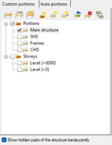
The workflow starts in the Portions Manager, where you can manually group structural members, frames, columns, beams, bracings into Custom Portions. These are fully user-defined and, importantly, only these custom portions can be directly used for analysis. This allows you to isolate exactly the structural subsystem you want to investigate, without being constrained by the full model.
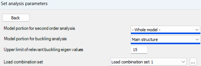
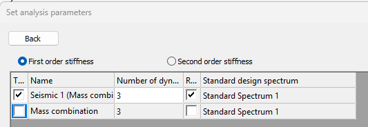
Once a portion is defined, it can be selected in the Analysis Settings, where you can choose whether second-order and buckling analyses should be performed on the entire model or only on the selected portion. The solver will then consider only that subset of elements when assembling the stiffness matrix and evaluating stability behavior.
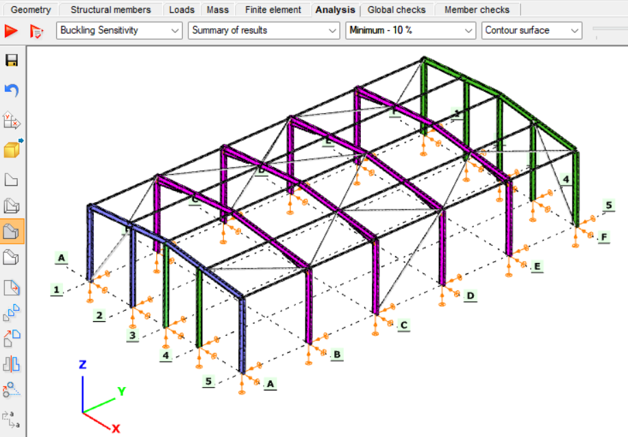
Running these analyses on specific portions has clear engineering advantages. Second-order effects and buckling phenomena are often governed by local structural behavior, such as a critical frame, a bracing system, or a column group, rather than the entire structure. By isolating these regions, you can:
- reduce computational effort and analysis time, especially for large models
- focus on the most critical load paths and instability mechanisms
- perform faster iterations during design refinement
- avoid unnecessary influence from non-relevant parts of the structure
This targeted approach leads to more efficient and controlled stability analysis, particularly when investigating sensitive or highly utilized structural components.
Download the example model and try it!
Download modelIf you haven’t tried Consteel yet, request a trial for free!
Try Consteel for freeIs a single dominant vibration mode sufficient, or should multiple vibration modes be considered in seismic analysis?
Steel portal frames are frequently used in industrial and logistics buildings as primary load-bearing structures. Their seismic behavior is strongly influenced by the stiffness of the roof diaphragm and by the interaction between the main portal frames and secondary structural subsystems such as endwalls.
In seismic design, engineers often assume that the global response of such buildings can be represented by a single dominant vibration mode. This assumption is valid when the roof diaphragm is sufficiently rigid and the first transverse mode mobilizes most of the structural mass. However, when the diaphragm is flexible or when different structural parts participate in different vibration modes, higher modes may also contribute to the seismic response.
This article investigates how the choice between a single-mode and a multi-modal approach affects the seismic design of steel halls modeled in Consteel. Through a comparative example, the study demonstrates the implications of different modal combination techniques and discusses how reliable internal forces can be obtained while maintaining compatibility with stability verification procedures according to EN 1993-1-1.
Case with a Rigid Roof Diaphragm
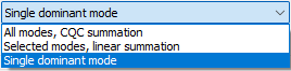
Single dominant mode
If a building is designed with a sufficiently rigid roof diaphragm, a single transverse vibration mode is typically able to mobilize close to 90% of the total participating mass. In such cases, the Single dominant mode method is an efficient and preferred design method.
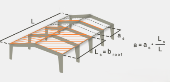
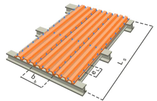
A rigid roof diaphragm can be achieved by:
- Using an adequate trapezoidal steel deck, modeled in Consteel either
- as a Shear Field with a high shear stiffness parameter (“S” value), or
- by introducing equivalent dummy roof bracing diagonals with rod diameters calibrated to reproduce the diaphragm shear stiffness.
- Alternatively, real bracing elements may be added along the sidewall columns or from the eaves to the ridge along the building length.
Case without a Rigid Roof Diaphragm
If a rigid diaphragm is intentionally not assumed, a single vibration mode will generally not represent the full seismic response in the transverse direction.
Single dominant mode
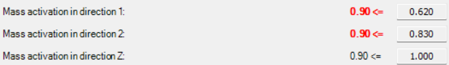
A dynamic eigenvalue analysis is first performed to determine the natural vibration modes of the structure. In Consteel, this analysis calculates the eigenfrequencies and corresponding mode shapes based on the structural stiffness and mass distribution, considering both the elastic stiffness and second-order geometric stiffness of the structure. The first three vibration modes are then evaluated for their mass participation in the transverse direction.
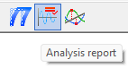
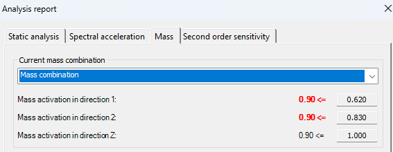
After the calculation, the mass participation for each principal direction (X, Y, and Z) can be viewed in the Analysis tab under the Analysis report, in the Mass section. In the examined case:
gateIntroduction
This article presents the calculation method for determining the buckling resistance of a pinned column with intermediate restraints in accordance with Eurocode standards. The procedure is based on an example from the Access Steel design examples collection and is compared with the calculation process implemented in Consteel’s steel member design functions, specifically within the Member Checks module.
In the following sections, a step-by-step guide is provided to demonstrate how the member check functionality can be applied to simple cases, highlighting both methodology and practical usage.
Input Data for the Example
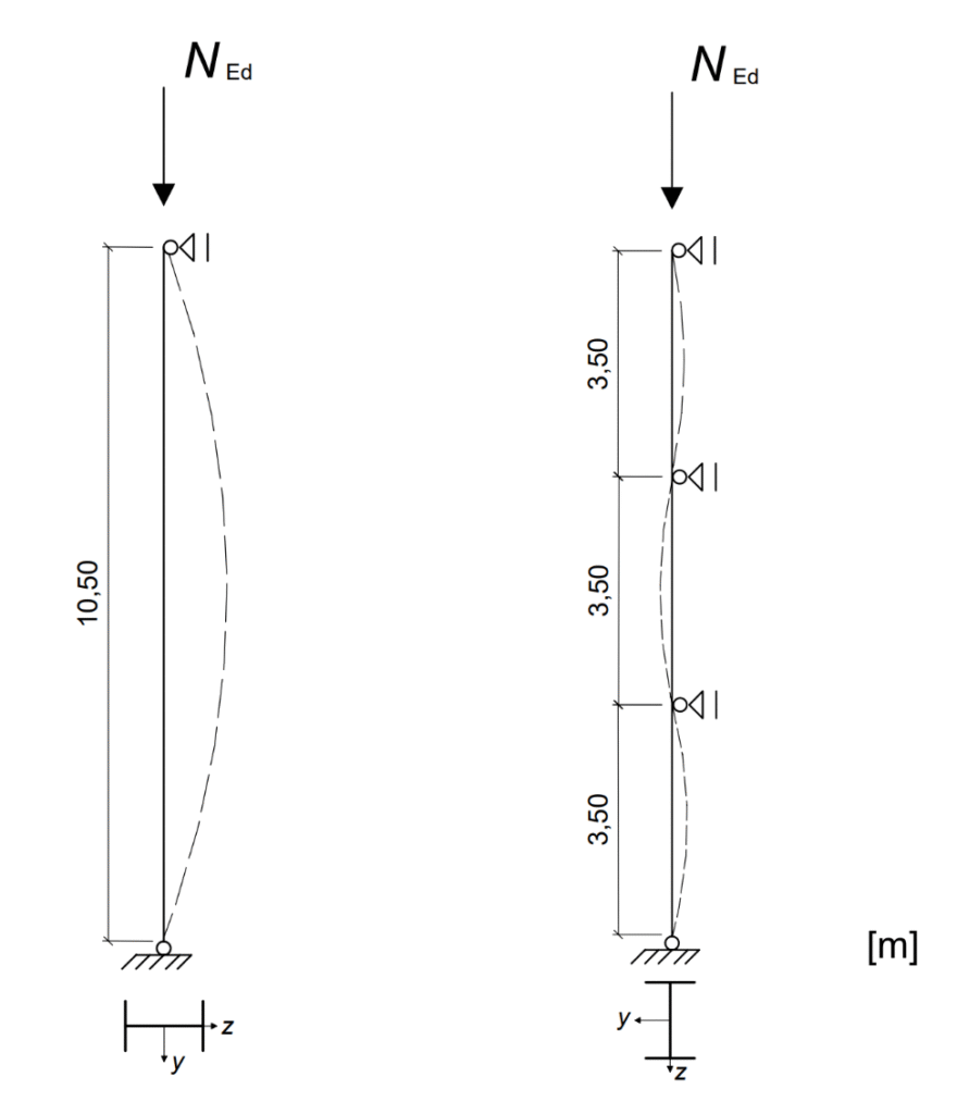
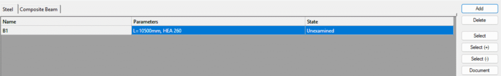
The example considers a pinned column in a multi-storey building, subjected to a design axial force of $N_{Ed}$ = 1000 kN. The column has a total length of 10.50 m and is laterally restrained about the y–y axis at intervals of 3.50 m.
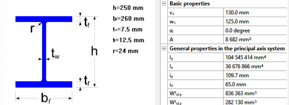
The member is a rolled HEA 260 section made of S235 steel. The cross-section is classified as Class 1. The geometric properties of the section are: height h = 250 mm, width b = 260 mm, web thickness $t_w$ = 7.5 mm, flange thickness $t_f$ = 12.5 mm, and fillet radius r = 24 mm. The cross-sectional area is A = 86.8 cm², with moments of inertia $I_y$ = 10450 cm⁴ and $I_z$ = 3668 cm⁴.
The material properties are defined according to EN 1993-1-1. Since the maximum thickness is less than 40 mm, the yield strength is taken as $I_y$ = 235 N/mm². The partial safety factors are γM0 = 1.0 and γM1 = 1.0.
Determining Design Buckling Resistance of a Compression Member
The design buckling resistance of the column $N_{b,Rd}$ is evaluated by determining the reduction factor χ for both principal buckling directions. This requires the calculation of the elastic critical forces $N_{cr}$, which form the basis for identifying the governing buckling mode.
Elastic critical force for the relevant buckling mode $N_{cr}$
The Young’s modulus is taken as $E=210000 \frac{N}{mm^2}$. The buckling lengths in the respective planes are $L_{cr,y} = 10.50m$ for buckling about the y–y axis and $L_{cr,z} = 3.50m$ for buckling about the z–z axis. Observe that the buckling lengths for the strong and weak axes differ according to the support conditions, which must be determined by the engineer in manual calculations.
$$N_{cr,y}=\frac{π^2*E*I_{y}}{L_{cr,y^2}}=1964.5 kN$$
$$N_{cr,z}=\frac{π^2*E*I_{z}}{L_{cr,z^2}}=6206.0 kN$$
In Consteel, the elastic critical force for the relevant buckling mode can be determined using the Individual Member Design approach. This is accessible in the Member Checks tab under the Steel module, where selected members can be added and evaluated.

Once a member is selected, the analysis results are automatically loaded, provided that first- or second-order analysis results are available. Ensure that the analysis has been run in the Analysis tab and the cross section check on the Global ckecks tab before proceeding to the Member Checks section.
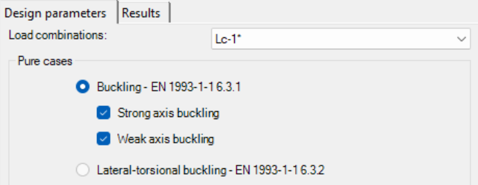
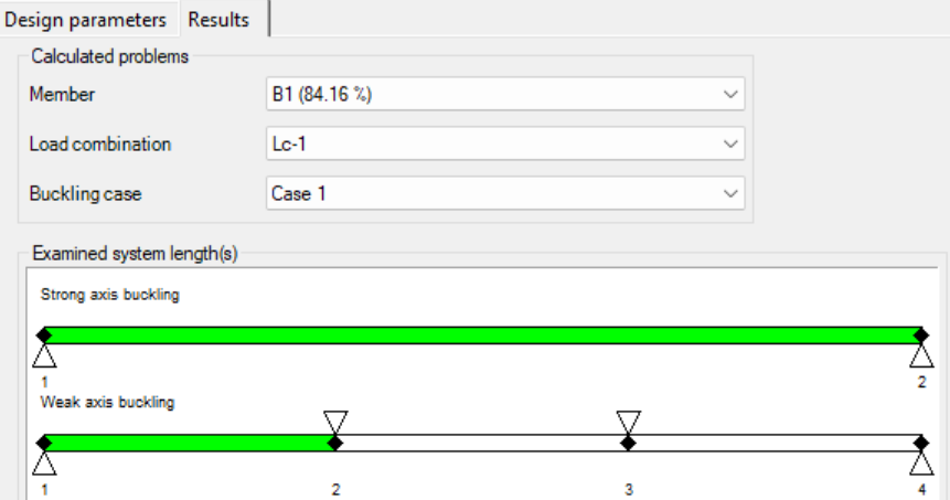
For the pinned column with intermediate restraints, the relevant buckling cases, strong and weak axis, are selected, and the dominant load combination is automatically indicated with a *. Consteel identifies the intermediate restraints separately for each direction and divides the member into segments accordingly to help determine the correct buckling lengths.
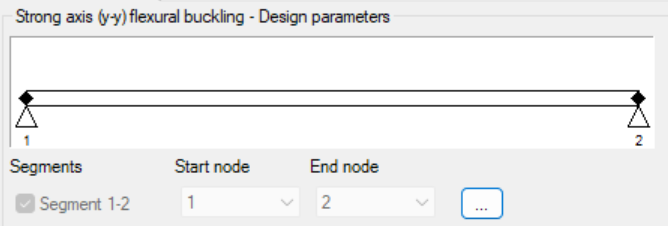
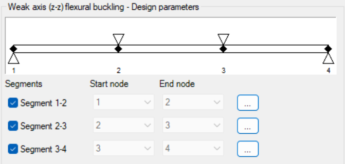
Design parameters for each segment are set with the three-dot icon:
At this step, users must verify the assigned values. By default, the first value is applied, and the correct buckling shape or effective length factor should be confirmed based on engineering judgment.
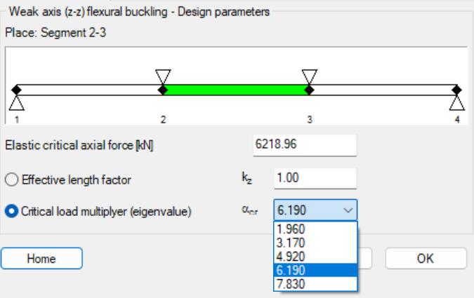
In order to use the critical load multiplier selection option, make sure to perform the calculation first:


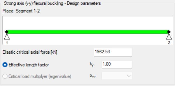
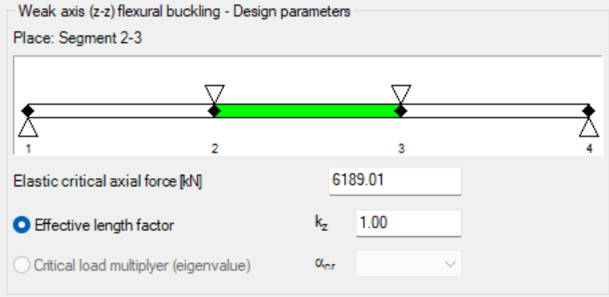
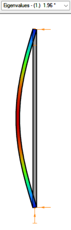
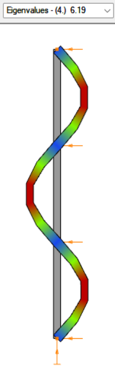
In order to check whether the correct critical load multiplier was selected, you can examine the effective length factor, which is calculated based on it (in this case, it is 1 for both directions). In our example, the relevant buckling shapes for the y–y and z–z directions are as follows:
The elastic critical force $N_{cr}$ is calculated automatically, regardless of whether the effective length factor was entered manually or the critical load multiplier was selected.
| Access Steel – manual calculation | Consteel using the effective length factor | Consteel using the critical load multiplier | |
| $N_{cr,y}$ | 1964.5 kN | 1962.53 kN | 1973.76 kN |
| $N_{cr,z}$ | 6206.0 kN | 6189.01 kN | 6218.96 kN |
Once all parameters are defined, the design check is executed by clicking the Check button, and the results are displayed.
Results can be reviewed and filtered by member, load combination, and buckling case. Lateral-torsional buckling checks follow a similar procedure, with segment boundaries adjustable and critical moments calculated either analytically or using the critical load multiplier.
Non-dimensional slenderness
In order to determine the reduction factor, the non-dimensional slenderness λ must be calculated based on the elastic critical force corresponding to the relevant buckling mode.
$$\overline{\lambda_y} = \sqrt{\frac{A*f_y}{N_{cr,y}}}=\sqrt{\frac{86.8*23.5}{1965}}=1.016$$
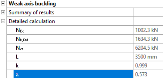
$$\overline{\lambda_z} = \sqrt{\frac{A*f_z}{N_{cr,z}}}=\sqrt{\frac{86.8*23.5}{6206}}=0.573$$
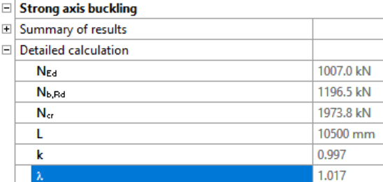
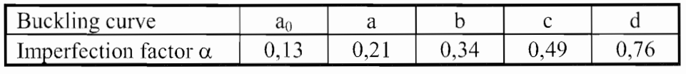
In Consteel, the detailed calculations for strong and weak axis buckling can be reviewed separately on the Results tab:
Reduction factor
For axial compression, the value of χ corresponding to the relevant non-dimensional slenderness $\overline{\lambda}$ should be determined from the appropriate buckling curve in accordance with EN 1993-1-1 §6.3.1.2.
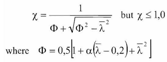
For $\frac{h}{b}= \frac{250mm}{260mm} = 0.96 < 1.2$ and $t_f = 12.5 mm< 100 mm$
- buckling about axis y-y, buckling curve b, imperfection factor $\alpha=0.34$
$$\varphi_y=0.5*[1+0.34(1.019-0.2)+1.019^2]=1.158$$
$$\chi_y=\frac{1}{1.158+\sqrt{1.158^2-1.019^2}}=0.585$$
- buckling about axis z-z, buckling curve c, imperfection factor $\alpha=0.49$
$$\varphi_y=0.5*[1+0.49(0.573-0.2)+0.573^2]=0.756$$
$$\chi_y=\frac{1}{0.756+\sqrt{0.756^2-0.573^2}}=0.801$$
$$\chi=min(\chi_y;\chi_z)$$
$$\chi=0.585<1.00$$
Design buckling resistance of a compression member
$$N_{b,Rd}=\chi*\frac{A*f_y}{\gamma_{M1}}=0.585*\frac{86.8*23.5}{1.0}=1193 kN$$
$$\frac{N_Ed}{N_{b,Rd}}=\frac{1000}{1193}=0.84<1.00$$
Conclusion
This example demonstrates the application of the isolated member approach for a simple compression member. For more complex cases or alternative stability verification methods, such as the imperfection approach or the general method, refer to the dedicated article on stability design methods, where their principles and applications are discussed in detail.
Download modelProgram verzió: Consteel 17; Build 3303
Tervezés célja, tervezési szabvány kiválasztása
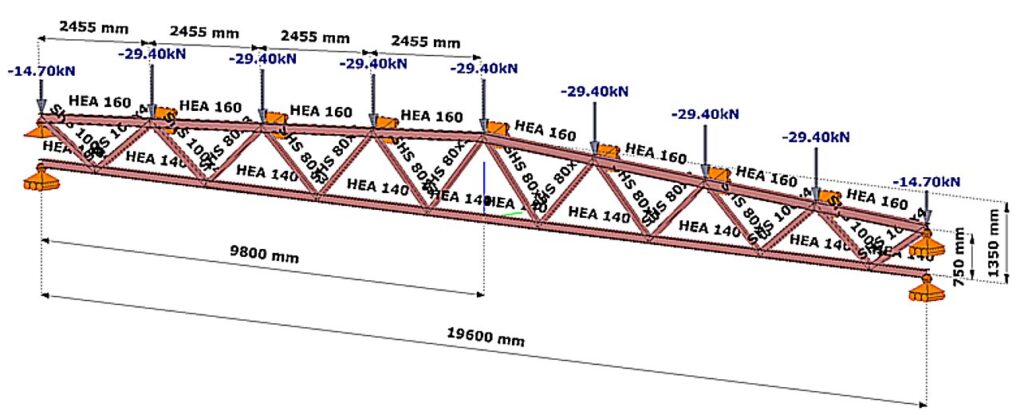
A jelen tervezési segédlet a kezdő ConSteel 17 felhasználó számára egy kéttámaszú rácsos tartó tervezését mutatja be, lépésről lépésre. Az építészeti koncepcionális tervből ismert a megtervezendő rácsos tartó geometriai kialakítása (1. ábra). A koncepció szerint a rácsos tartó övei HEA120 típusú melegen hengerelt szelvényből készülnek, míg a rácsrúdjai hidegen alakított SHS80x4 szelvényből. A jelen segédletnek a csomópontok tervezése nem része.

Ismert, hogy a szerkezettervezés mindig valamely szabvány, illetve annak változata szerint történik. A szabvány kiválasztása új modell létrehozásakor a Project centerben a Tervezési szabvány menüből választható, vagy később a Szabványok rendszerfül [S1] kiválasztó paneljében módosítható (2. ábra).

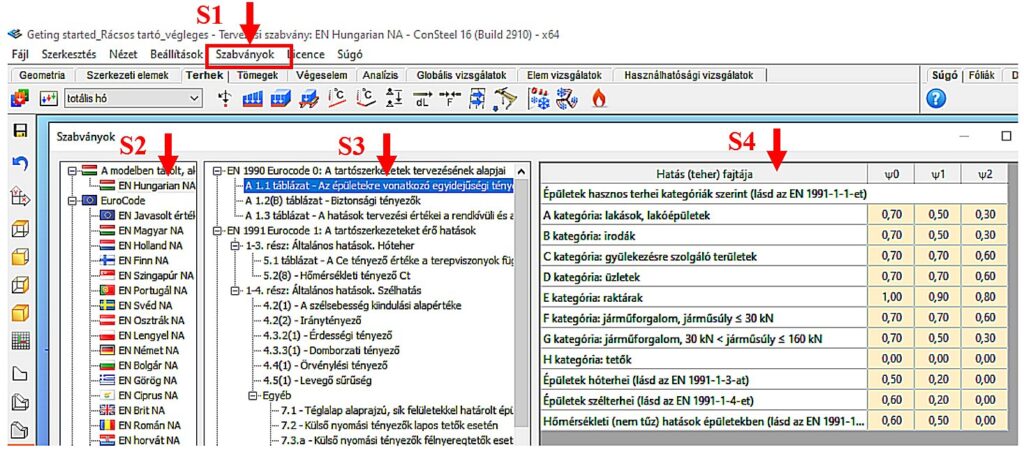
Az alkalmazni kívánt tervezési szabvány a panel bal oldali listájából választható ki. Jelen esetben az EN Hungarian NA opciót [S2] választjuk (MSz EN Magyar Nemzeti melléklet). A kiválasztott szabvány által alkalmazott paraméterek a középső tartalomjegyzék megfelelő sorának kiválasztásával érthető el, a jobb oldali táblázatban [S4]. A 2. ábrán az EC0 szabvány 1.1 táblázatának megfelelő egyidejűségi tényezők kerültek kiválasztásra, amely paramétereket a jobb oldali táblázat mutatja meg.
Szerkesztő raszter beállítása
Először állítsuk be a raszter méretét a szerkezet fesztávjának megfelelően. Ehhez alkalmazzuk a baloldalon található eszközcsoport megfelelő gombját [1], amelynek hatására megjelenik a Raszterháló és koordinátarendszer beállító panel (2. ábra).
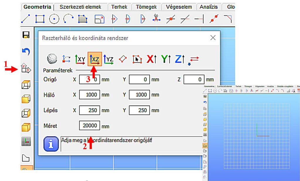
Például a 19.6m hosszú tartó esetén a Méret ablak tartalmát 20000 milliméterre állíthatjuk [2]. A beállítás aktualizálásához nyomjuk meg az Enter-t, vagy zárjuk be az ablakot. A fenti beállítás esetén a raszter X és Y irányban 20 méter széles lesz, a raszter vonalak sűrűsége 1000 mm, a lépésközök 250 mm. A rácsos tartó modellt célszerű az X-Z globális koordináta síkban felvenni, tehát a szerkesztő rasztert el kell fordítanunk az X-Z síkba. Ehhez válasszuk XZ sík opciót [3].
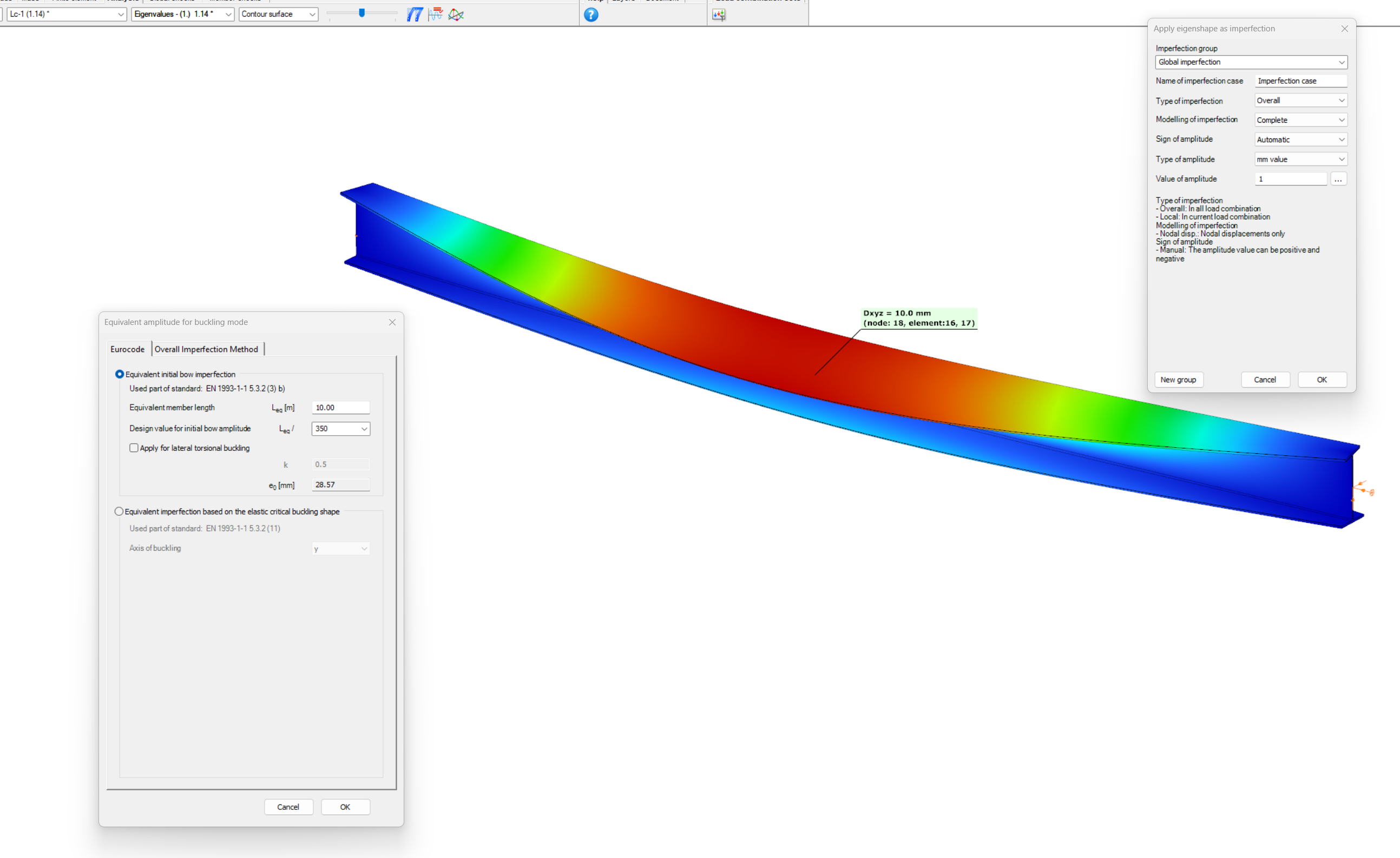
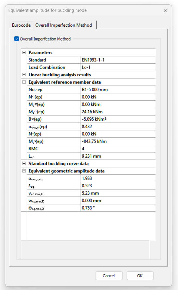
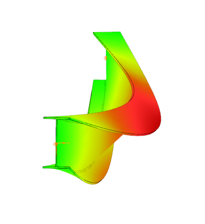
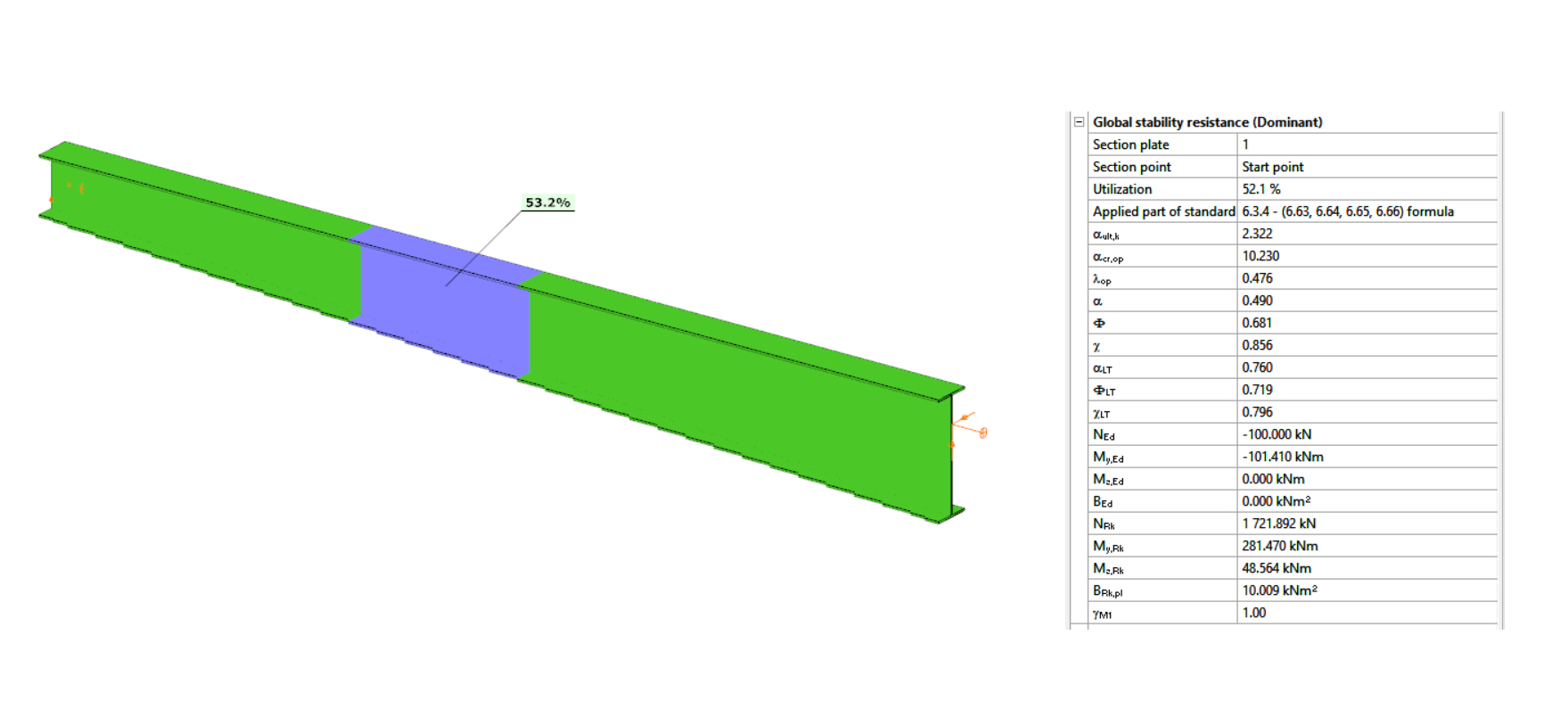
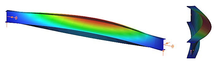
gateConsteel recommends to use the General Method from EN 1993-1-1 for the evaluation of out-of-plane strength of members and sturctures. In addition, the scaled imperfection based 2nd order approach is available.
Did you know, that when linear buckling eigenform affine imperfections are used, Consteel can scale automatically the selected eigenmodes to perform a Eurocode compatible design? And you can even combine several imperfections?
Download the example model and try it!
Bending:
Download modelCopmression:
Download modelIf you haven’t tried Consteel yet, request a trial for free!
Try Consteel for free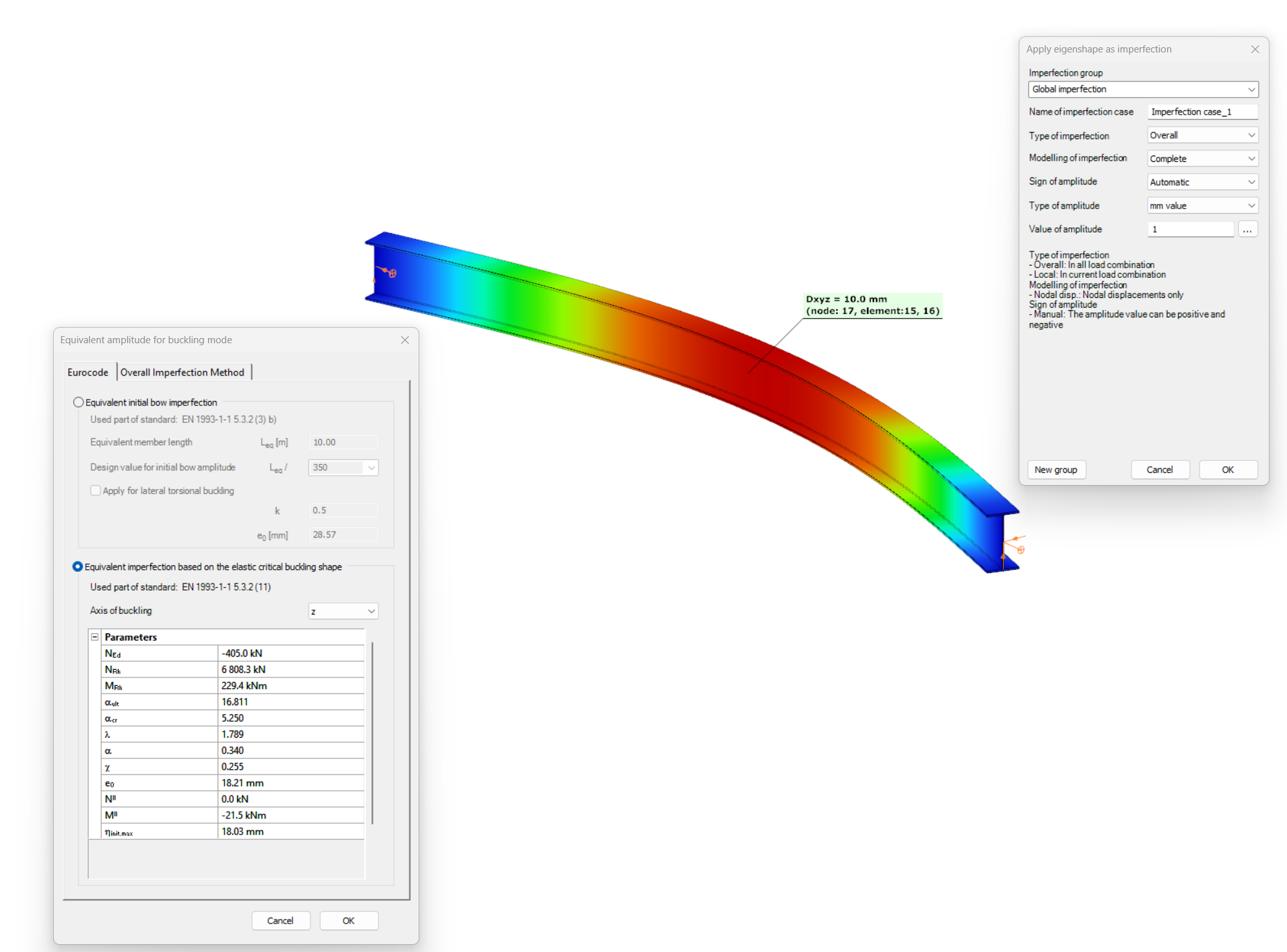
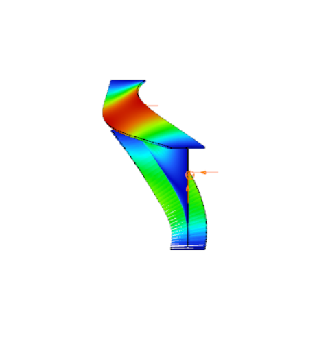
Have you ever heard about the ‘General Method’? This is an alternative design method to consider the interaction of axial compression with major-axis bending for general buckling situations, where the main interaction formulas are not applicable.
This basically includes every member with monosymmetric or asymmetric cross-sections or with cross-sections not uniform along the length (welded tapered sections) or laterally stabilized by sheeting or anything else without providing full fork supports.
Did you know, that the General Method is fully supported by Consteel and provides an automated buckling verification possibility? Of course, for the use of the General Method in a general case the traditional 12DOF beam finite elements are not applicable. But the special 14DOF beam elements used by Consteel are perfectly compatible?
Download the example model and try it!
Download modelIf you haven’t tried Consteel yet, request a trial for free!
Try Consteel for free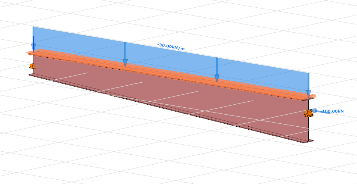
Bevezetés
Amennyiben a síkban hajlított gerenda szabadon elmozdulhat és elcsavarodhat a két támaszpontja között, akkor a lehajlás mellett hirtelen merőleges elmozdulás és elcsavarodás jöhet létre: a gerenda kifordul a síkjából. Ezt a jelenséget szemlélteti az 1. ábra, amely egy kéttámaszú, az erős tengely körül hajlított I keresztmetszetű gerendát mutat: a függőleges síkban történő hajlítás során, amikor a nyomaték elér egy kritikus értéket, a gerenda hirtelen oldalirányban elmozdul és elfordul a két támasz között. Ez a jelenség a kifordulás, amely stabilitásvesztési mód a tökéletes gerendára és a valódi gerendára egyaránt vonatkozhat.
A gerenda kifordulással szembeni méretezése teljes mértékben analóg a nyomott oszlop kihajlási elleni méretezésével. Az analógiát az 1. táblázat szemlélteti, ahol feltüntettük a kihajlási és a kifordulási ellenállást befolyásoló, egymásnak megfelelő paramétereket.
| Kihajlás | Kifordulás |
|---|---|
| tervezési nyomóerő ($N_{Ed}$) | tervezési nyomaték ($M_{Ed}$) |
| kritikus erő ($N_{cr}$) | kritikus nyomaték ($M_{cr}$) |
| kihajlási karcsúság ($\frac{}{\lambda}$) | kifordulási karcsúság ($\frac{}{\lambda}_{LT}$) |
| kihajlási csökkentő tényező ($\chi$) | kifordulási csökkentő tényező ($\chi_{LT}$) |
| kihajlási ellenállás ($N_{b,Rd}$) | kifordulási ellenállás ($M_{b,Rd}$) |
A tökéletes gerenda kritikus nyomatékát a My,Edtervezési hajlítónyomaték-diagram maximális értékének helyén kell meghatározni. Kétszeresen szimmetrikus I keresztmetszet esetén:
$$M_{cr}=C_1\frac{\pi^2EI_z}{(k_z⋅L)^2}\left[\frac{I_\omega }{I_z}+ \frac{(k_zL)^2GI_t}{\pi^2EI_z}\right] ^{0.5} $$
ahol kz a keresztmetszet gyenge tengelye körüli befogási tényező, G a nyírási modulus, It és Iω pedig a keresztmetszet tiszta (St. Venant) és gátolt csavarási tehetetlenségi nyomatéka. A C1 tényező értéke a hajlító nyomatéki diagram alakjától függ, az értéke megfelelő táblázatokban és kézikönyvekben megtalálható. Konstans nyomatéki ábra esetén C1=1.0. A többi tervezési paraméter, különösen a $\chi_{LT}$ kifordulási csökkentő tényező képlete a figyelembe vett tervezési szabványtól függ.
Kifordulási ellenállás az EN1993-1-1 szerint
A hajlított gerenda kifordulás elleni méretezését (teherbírás-ellenőrzést) az EC3-1-1 szerint a következő lépésekben kell elvégezni:
gateRácsos tartó szerkezet méretezése
A rácsos tartók globális (rúdszerkezeti szintű) méretezése nem igényel különleges elméleti ismeretet: rendszerint a hajlítónyomatékok és a nyíróerők elhanyagolásával a rácsos tartók rudjait nyomott és/vagy húzott rúdként méretezzük. A nyomott rudak méretezését manapság modell alapú számítógépes eljárással hajtjuk végre. Ennek részleteit lásd a Nyomott rúd méretezése kihajlás ellen című tudásbázis anyagban. Itt csak a nyomott rudak kihajlási hosszának meghatározását mutatjuk be.
A nyomott rúd méretezésénél a legfontosabb paraméter a rúdkarcsúság:
$$\overline{\lambda}=\sqrt\frac{Af_y}{N_{cr}}$$
ahol
$$N_{cr}=\frac{\pi^2El}{(kL)^2}$$
ahol a k kihajlási hosszt (befogási tényezőt) az EN1993-1-1 szabvány, a kézi számítások megkönnyítése érdekében, az alábbiak szerint javasolja felvenni:
| Nyomott rúd típusa | Kihajlás iránya | k |
|---|---|---|
| övrúd | – tartó síkjában – tartó síkjára merőlegesen | 0.9 0.9 |
| rácsrúd | – tartó síkjában – tartó síkjára merőlegesen | 0.9 1.0 |
A modell alapú számítógépes eljárásokon alapuló szoftverek (pl. a Consteel szoftver) a fenti konzervatív szabály helyett az Ncr rugalmas kritikus erőt közvetlenül végeselemes numerikus módszerrel, a teljes rácsos tartó viselkedésének figyelembe vételével, határozzák meg. Az alábbi példával a szabvány által javasolt kézi méretezési eljárás és a modern, modell alapú numerikus eljárás eredményének viszonyát kívánjuk szemléltetni.
- Legyen a vizsgált rácsos tartó szerkezeti modellje az 1. ábrán látható Consteel modell.
- A feltűntetett teher feleljen meg a tartó mértékadó tervezési teherkombinációjának.
- Határozzuk meg a legjobban igénybe vett nyomott övrúd kihajlási hosszát végeselemes numerikus stabilitási analízis segítségével.
(Consteel szoftver)
Eljárások összehasonlítása
A számítás lépései a következők:
Rugalmas stabilitási analízis
A rugalmas modell stabilitási analízise megmutatja, hogy a rácsos szerkezet mértékadó stabilitásvesztési módját és az ahhoz tartozó αcr rugalmas kritikus teherszorzót (2. ábra).
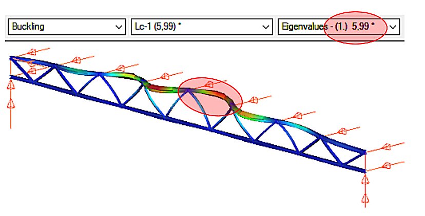
Láthatjuk, hogy a terhelés hatására a tökéletesen rugalmas modell felső öve oldalsó irányban kihajlást szenved. A teher, amely hatására a rugalmas kihajlás bekövetkezik, a kritikus teher, amelynek értékét a tervezési teher és az αcr=5.99 kritikus teherszorzó szorzata adja meg.
gateA nyomott rúd méretezésének fejlődése
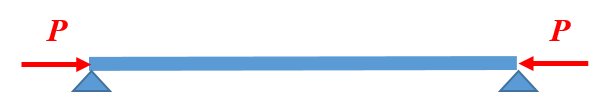
A rudakból épített acélszerkezetek (pl. rácsos tartók) egyik jellegzetes alkotó eleme a nyomott rúd. Nyomott rúdról akkor beszélünk, ha a rendszerint egyenes tengelyű szerkezeti elem központos P nyomóerővel terhelt (1. ábra).
A 2. ábra a nyomott rúd méretezésének fejlődését illusztrálja. Kezdetben (a régi időkben) az építőmesterek az évszázadok során felhalmozódott tapasztalati ismeretek alapján, amelyek mesterről tanítványra szálltak, állapították meg a különböző anyagú és méretű nyomott oszlopok teherbírását. Jelentős változást a klasszikus matematikai differenciálanalízis mérnöki alkalmazása hozott. Euler (1707-1783) svájci matematikus és fizikus megoldotta a nyomott rugalmas vonal kihajlásának problémáját, amely megoldás alkalmazható volt a rugalmas nyomott rúd megoldására (Euler erő). A mérnökök a következő évszázadokban felismerték, hogy az Euler erő csak bizonyos esetekben (elsősorban nagy karcsúságoknál) ad elfogadható közelítést a nyomott rúd valós teherbírására. Számos, az Euler képletnél fejlettebb megoldás született a nyomott rúd teherbírására, de jelentős változást csak a II. világháborút követő hatalmas szerkezetépítési konjunktúra hozott. A világ minden számottevő szerkezeti laboratóriumában sorra végezték a nyomott rúd kísérleteket, majd az eredményekből összeállítottak egy több mint kétezer kísérletből álló adatbázist. A nyomott rúd teherbírását az adatbázis alapján, a matematikai statisztika módszerével meghatározott képlettel adták meg.
Ez a módszertan a mai napig meghatározó: „a nyomott rúd méretezése az acélszerkezeti szakma politikai kérdése lett…”. Ezért a nyomott rúd méretezési elvének megértése a szerkezet-építőmérnök számára alapvető fontosságú.
Az ábra jobb oldala a jövőre is tartalmaz utalást. A tudományos kutatás szintjén már jelen, hogy a valós nyomott rúd teherbírását matematikai-mechanikai szimulációval is meg lehet határozni. Sőt, a közeljövőben minden eddigi ismeretet meghaladó adatbázisok hozhatók létre a szuperszámítógépek bevetésével. Egy ilyen gigantikus adatbázis alapján a mesterséges intelligencia felülírhatja az eddigi mérnöki tudást és módszertant, legalábbis elvben. A valóság viszont az, hogy a szerkezet-éptőmérnökség nem tartozik a húzóágazatok közé (mint például a hadipar vagy az autóipar), ezért ez az új méretezéselméleti váltás még egy jó ideig bizonyosan várat magára.

A továbbiakban a ma acélszerkezeti mérnöksége számra kiemelten fontos Euler erőt és a kísérleti alapú szabványos méretezési formulát tárgyaljuk részletesen.
Az ideális nyomott rúd teherbírása: az Euler erő
Tételezzük fel, hogy az alábbi ábrán látható csuklósan megtámasztott nyomott rúd rendelkezik az alábbi tulajdonságokkal:
- tökéletesen egyenes,
- az anyaga tökéletesen lineárisan rugalmas,
- központosan nyomott.
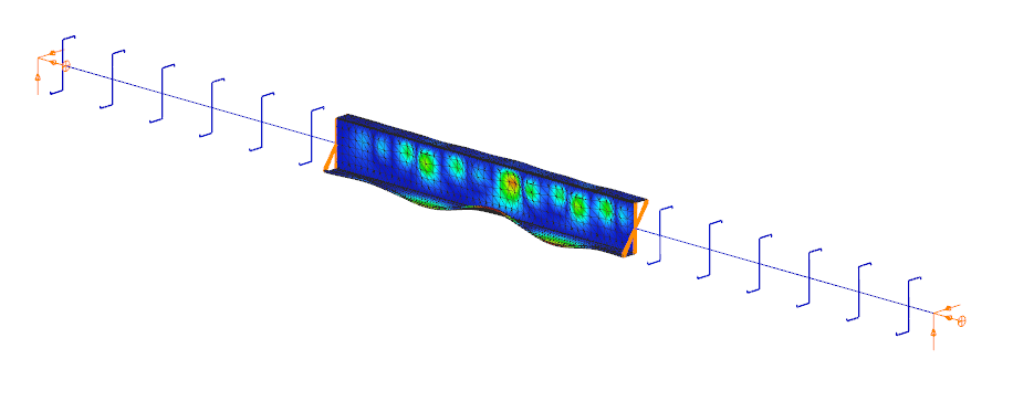
A fenti feltételekkel végezzük el a nyomott rúd kísérletet a Consteel szoftver segítségével: futtassuk a lineáris kihajlási analízis (Linear Buckling Analysis, LBA) számítást. Az eredményt a 3. ábra szemlélteti.
gateDid you know that you could use Consteel to perform dual analysis with 7DOF beam and/or shell elements?
With two advanced features, Superbeam and Convert members to plates, you can choose the approach that best suits your project needs, whether you’re focused on modeling efficiency or detailed analysis.
The Superbeam function offers a smart, adaptive way to handle structural members. It enables you to model with the simplicity of standard 7DOF beam elements while allowing you to switch to a more detailed shell-based analysis for specific members whenever needed.
Once the structure is modeled using beam elements, you can select how each member is analyzed:
- Using the beam model, which applies Consteel’s proven 7DOF beam elements along with its comprehensive design tools.
- Or using a shell model, which is automatically generated for selected members. This shell model includes detailing features such as web cutouts and stiffeners, fully integrated into the global analysis model.
This dual approach is fully adaptive. You can continue modifying your model using beam elements and switch between analysis modes as required, offering both speed and precision within the same workflow.
For a complete overview of how to activate and manage Superbeam functionality, refer to the documentation:
Superbeam – Consteel Manual


When you need complete control over geometry and mesh, or when shell analysis alone is not sufficient, Consteel provides the Convert members to plates function. This tool allows you to manually transform selected members into actual plate elements, enabling detailed modeling from the start.
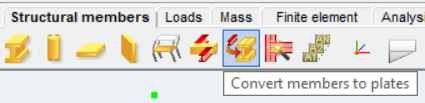
Unlike the automatic conversion used in Superbeam, this method performs a permanent, non-reversible transformation (though undo is available during the session). It supports a wide range of section types, including hot-rolled, cold-formed, and welded profiles.
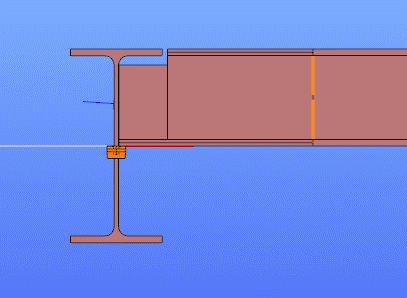
The conversion process preserves and adapts existing connections, eccentricities, loads, and supports. Where needed, rigid bodies and constraint elements are added to maintain structural continuity. These constraints ensure proper transfer of deformations, including warping, between the new plate model and the rest of the structure.
This function is especially useful in cases where precision is critical, such as modeling joints, fabrication-specific details, or complex load interactions.
To learn more, see the full guide here:
Convert Members to Plates – Consteel Manual
Both Superbeam and Convert members to plates serve different purposes, depending on the level of detail and control required in your model:
| Feature | Superbeam | Convert members to plates |
| Workflow | Beam modeling with optional shell analysis | Full plate modeling from the beginning |
| Conversion | Automatic and reversible | Manual and permanent |
| Suitable For | Flexibility in analysis, quick modeling | Full control, high-detail requirements |
| Supported Sections | Welded I and H profiles | Hot-rolled, cold-formed, and welded sections |
| Detailing Support | Cutouts and stiffeners (in shell analysis) | Full geometric detailing, including transitions |
| Design Integration | Integrated with beam-based design tools | Suitable for fabrication-level modeling |
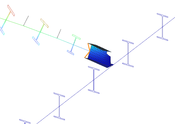
In Superbeam, constraint elements are generated automatically to connect converted shell elements to other members, such as bars. During member-to-shell conversion, these elements link the FE shell nodes to the rest of the model, ensuring accurate deformation transfer.
If the convert members to plate function is applied directly to beam elements, rigid bodies are created at their ends, which is useful for analyzing local behavior but does not transfer warping deformations. If the beam is first converted to a shell and then to plates, hinged rigid edges are placed along the plate boundaries. This arrangement, combined with constraint elements, transfers not only in-plane and out-of-plane deformations but also warping between the shell and the rest of the structure.
Download the example model and try it!
Download modelIf you haven’t tried Consteel yet, request a trial for free!
Try Consteel for free