Bevezetés
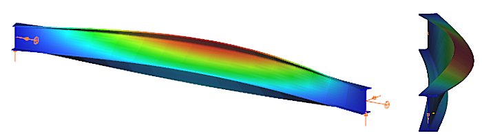
Amennyiben a síkban hajlított gerenda szabadon elmozdulhat és elcsavarodhat a két támaszpontja között, akkor a lehajlás mellett hirtelen merőleges elmozdulás és elcsavarodás jöhet létre: a gerenda kifordul a síkjából. Ezt a jelenséget szemlélteti az 1. ábra, amely egy kéttámaszú, az erős tengely körül hajlított I keresztmetszetű gerendát mutat: a függőleges síkban történő hajlítás során, amikor a nyomaték elér egy kritikus értéket, a gerenda hirtelen oldalirányban elmozdul és elfordul a két támasz között. Ez a jelenség a kifordulás, amely stabilitásvesztési mód a tökéletes gerendára és a valódi gerendára egyaránt vonatkozhat.
A gerenda kifordulással szembeni méretezése teljes mértékben analóg a nyomott oszlop kihajlási elleni méretezésével. Az analógiát az 1. táblázat szemlélteti, ahol feltüntettük a kihajlási és a kifordulási ellenállást befolyásoló, egymásnak megfelelő paramétereket.
| Kihajlás | Kifordulás |
|---|---|
| tervezési nyomóerő ($N_{Ed}$) | tervezési nyomaték ($M_{Ed}$) |
| kritikus erő ($N_{cr}$) | kritikus nyomaték ($M_{cr}$) |
| kihajlási karcsúság ($\frac{}{\lambda}$) | kifordulási karcsúság ($\frac{}{\lambda}_{LT}$) |
| kihajlási csökkentő tényező ($\chi$) | kifordulási csökkentő tényező ($\chi_{LT}$) |
| kihajlási ellenállás ($N_{b,Rd}$) | kifordulási ellenállás ($M_{b,Rd}$) |
A tökéletes gerenda kritikus nyomatékát a My,Edtervezési hajlítónyomaték-diagram maximális értékének helyén kell meghatározni. Kétszeresen szimmetrikus I keresztmetszet esetén:
$$M_{cr}=C_1\frac{\pi^2EI_z}{(k_z⋅L)^2}\left[\frac{I_\omega }{I_z}+ \frac{(k_zL)^2GI_t}{\pi^2EI_z}\right] ^{0.5} $$
ahol kz a keresztmetszet gyenge tengelye körüli befogási tényező, G a nyírási modulus, It és Iω pedig a keresztmetszet tiszta (St. Venant) és gátolt csavarási tehetetlenségi nyomatéka. A C1 tényező értéke a hajlító nyomatéki diagram alakjától függ, az értéke megfelelő táblázatokban és kézikönyvekben megtalálható. Konstans nyomatéki ábra esetén C1=1.0. A többi tervezési paraméter, különösen a $\chi_{LT}$ kifordulási csökkentő tényező képlete a figyelembe vett tervezési szabványtól függ.
Kifordulási ellenállás az EN1993-1-1 szerint
A hajlított gerenda kifordulás elleni méretezését (teherbírás-ellenőrzést) az EC3-1-1 szerint a következő lépésekben kell elvégezni:
gateA nyomott rúd méretezésének fejlődése
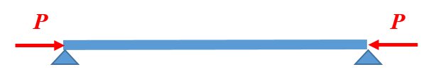
A rudakból épített acélszerkezetek (pl. rácsos tartók) egyik jellegzetes alkotó eleme a nyomott rúd. Nyomott rúdról akkor beszélünk, ha a rendszerint egyenes tengelyű szerkezeti elem központos P nyomóerővel terhelt (1. ábra).
A 2. ábra a nyomott rúd méretezésének fejlődését illusztrálja. Kezdetben (a régi időkben) az építőmesterek az évszázadok során felhalmozódott tapasztalati ismeretek alapján, amelyek mesterről tanítványra szálltak, állapították meg a különböző anyagú és méretű nyomott oszlopok teherbírását. Jelentős változást a klasszikus matematikai differenciálanalízis mérnöki alkalmazása hozott. Euler (1707-1783) svájci matematikus és fizikus megoldotta a nyomott rugalmas vonal kihajlásának problémáját, amely megoldás alkalmazható volt a rugalmas nyomott rúd megoldására (Euler erő). A mérnökök a következő évszázadokban felismerték, hogy az Euler erő csak bizonyos esetekben (elsősorban nagy karcsúságoknál) ad elfogadható közelítést a nyomott rúd valós teherbírására. Számos, az Euler képletnél fejlettebb megoldás született a nyomott rúd teherbírására, de jelentős változást csak a II. világháborút követő hatalmas szerkezetépítési konjunktúra hozott. A világ minden számottevő szerkezeti laboratóriumában sorra végezték a nyomott rúd kísérleteket, majd az eredményekből összeállítottak egy több mint kétezer kísérletből álló adatbázist. A nyomott rúd teherbírását az adatbázis alapján, a matematikai statisztika módszerével meghatározott képlettel adták meg.
Ez a módszertan a mai napig meghatározó: „a nyomott rúd méretezése az acélszerkezeti szakma politikai kérdése lett…”. Ezért a nyomott rúd méretezési elvének megértése a szerkezet-építőmérnök számára alapvető fontosságú.
Az ábra jobb oldala a jövőre is tartalmaz utalást. A tudományos kutatás szintjén már jelen, hogy a valós nyomott rúd teherbírását matematikai-mechanikai szimulációval is meg lehet határozni. Sőt, a közeljövőben minden eddigi ismeretet meghaladó adatbázisok hozhatók létre a szuperszámítógépek bevetésével. Egy ilyen gigantikus adatbázis alapján a mesterséges intelligencia felülírhatja az eddigi mérnöki tudást és módszertant, legalábbis elvben. A valóság viszont az, hogy a szerkezet-éptőmérnökség nem tartozik a húzóágazatok közé (mint például a hadipar vagy az autóipar), ezért ez az új méretezéselméleti váltás még egy jó ideig bizonyosan várat magára.

A továbbiakban a ma acélszerkezeti mérnöksége számra kiemelten fontos Euler erőt és a kísérleti alapú szabványos méretezési formulát tárgyaljuk részletesen.
Az ideális nyomott rúd teherbírása: az Euler erő
Tételezzük fel, hogy az alábbi ábrán látható csuklósan megtámasztott nyomott rúd rendelkezik az alábbi tulajdonságokkal:
- tökéletesen egyenes,
- az anyaga tökéletesen lineárisan rugalmas,
- központosan nyomott.
A fenti feltételekkel végezzük el a nyomott rúd kísérletet a Consteel szoftver segítségével: futtassuk a lineáris kihajlási analízis (Linear Buckling Analysis, LBA) számítást. Az eredményt a 3. ábra szemlélteti.
gateDid you know that you could use Consteel to Consider the shear stiffness of a steel deck as stabilization for steel members?
Download the example model and try it!
Download modelIf you haven’t tried Consteel yet, request a trial for free!
Try Consteel for free
Introduction
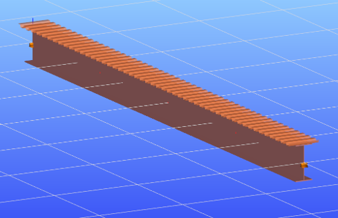
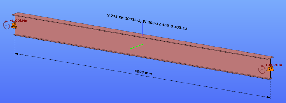
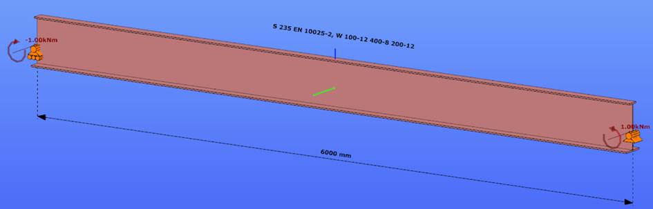
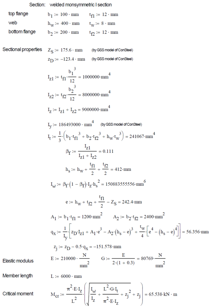
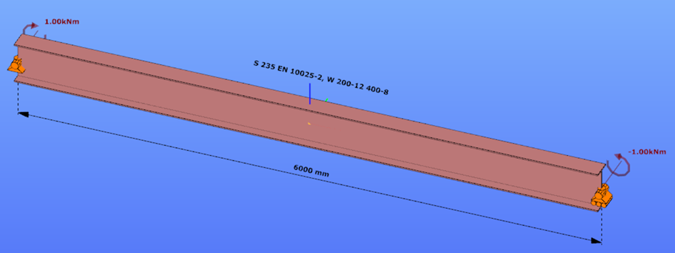
This verification example studies a simple fork supported beam member with welded section (flanges: 200-12 and 100-12; web: 400-8) subjected to bending about major axis. Constant bending moment due to concentrated end moments and triangular moment distribution from concentrated transverse force is examined for both orientations of the I-section. Critical moment and force of the member is calculated by hand and by the Consteel software using both 7 DOF beam finite element model and Superbeam function.
Geometry
Normal orientation – wide flange in compression
Constant bending moment distribution
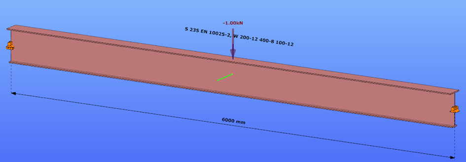
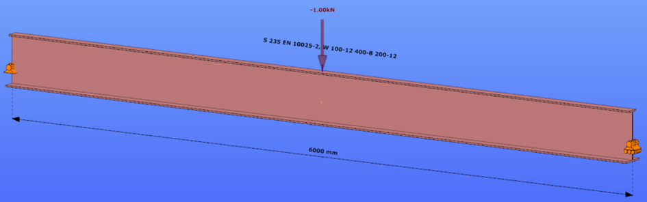
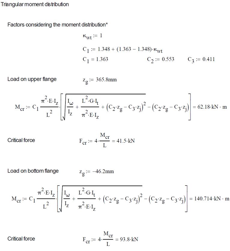
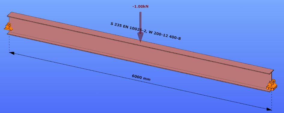
Triangular bending moment distribution – load on upper flange
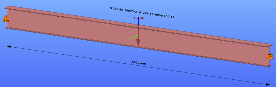
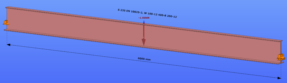
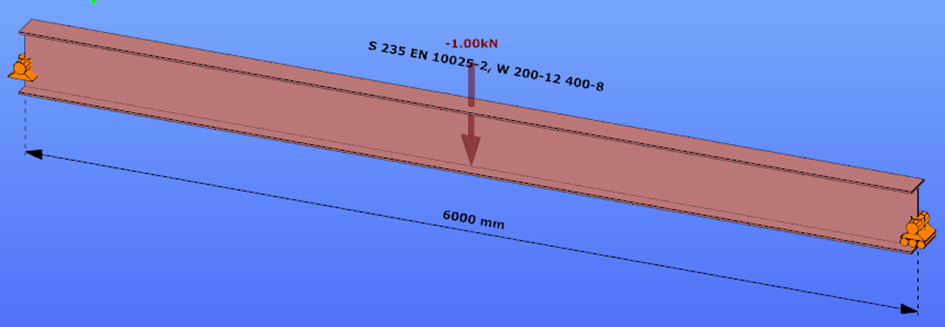
Triangular bending moment distribution – load on bottom flange
Reverse orientation – narrow flange in compression
Constant bending moment distribution
Triangular bending moment distribution – load on upper flange
Triangular bending moment distribution – load on bottom flange
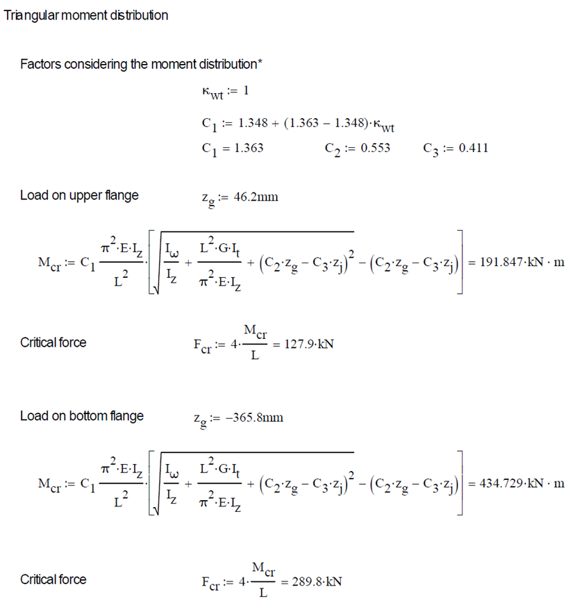
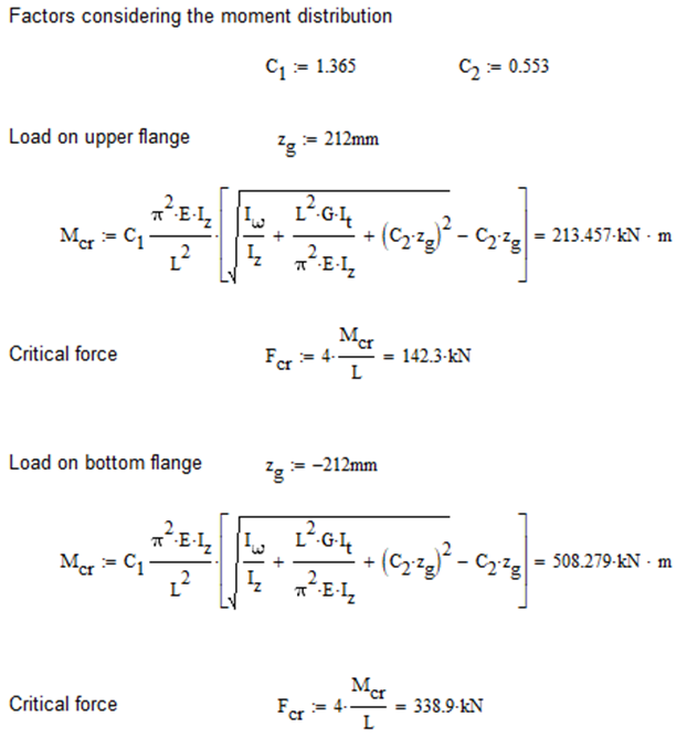
Calculation by hand
Factors to be used for analitical approximation formulae of elastic critical moment are taken from G. Sedlacek, J. Naumes: Excerpt from the Background Document to EN 1993-1-1 Flexural buckling and lateral buckling on a common basis: Stability assessments according to Eurocode 3 CEN / TC250 / SC3 / N1639E – rev2
Normal orientation – wide flange in compression
Constant bending moment distribution
Reverse orientation – narrow flange in compression
Computation by Consteel
Version nr: Consteel 15 build 1722
Normal orientation – wide flange in compression
Constant bending moment distribution
- 7 DOF beam element
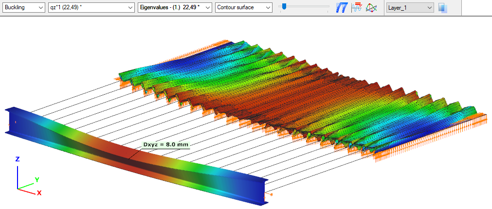
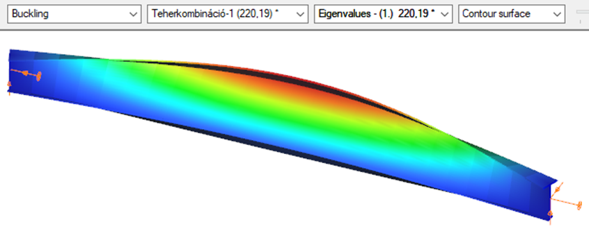
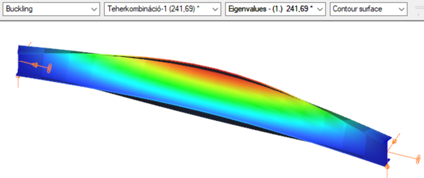
First buckling eigenvalue of the member which was computed by the Consteel software using the 7 DOF beam finite element model (n=25). The eigenshape shows lateral torsional buckling.
Superbeam
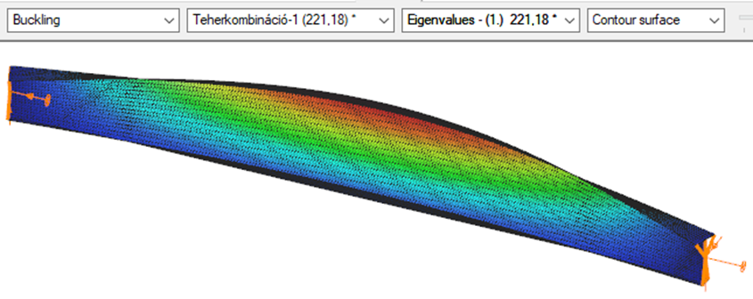
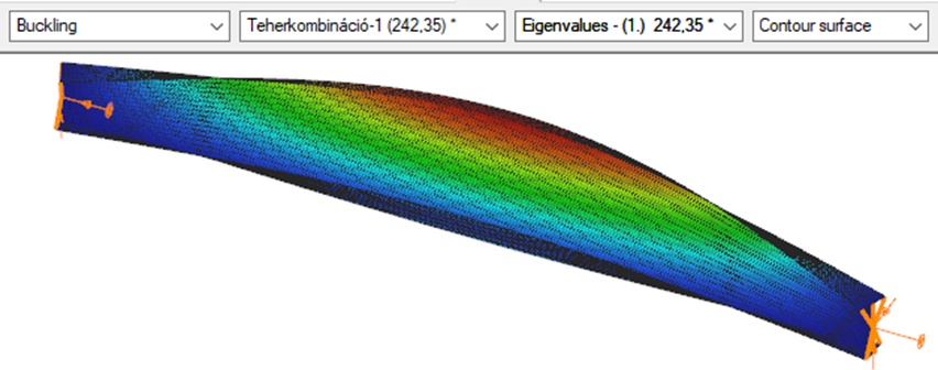
First buckling eigenvalue of the member which was computed by the Consteel software using the Superbeam function (δ=25).
Introduction
This verification example studies a simple fork supported beam member with welded section (flanges: 200-12; web: 400-8) subjected to bending about major axis. Constant bending moment due to concentrated end moments and triangular moment dsitribution from concentrated transverse force is examined. Critical moment and force of the member is calculated by hand and by the Consteel software using both 7 DOF beam finite element model and Superbeam function.
Geometry
Constant bending moment distribution
Triangular bending moment distribution – load on upper flange
Triangular bending moment distribution – load on bottom flange
Calculation by hand
Constant bending moment distribution

Triangular bending moment distribution
Computation by Consteel
Version nr: Consteel 15 build 1722
Constant bending moment distribution
7 DOF beam element
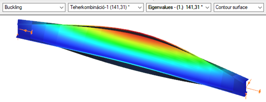
First buckling eigenvalue of the member which was computed by the Consteel software using the 7 DOF beam finite element model (n=16). The eigenshape shows lateral torsional buckling.
Superbeam
First buckling eigenvalue of the member which was computed by the Consteel software using the Superbeam function (δ=25).
Triangular bending moment distribution – load on upper flange
7 DOF beam element
First buckling eigenvalue of the member which was computed by the Consteel software using the 7 DOF beam finite element model (n=16).
Superbeam
First buckling eigenvalue of the member which was computed by the Consteel software using the Superbeam function (δ=25).

Triangular bending moment distribution – load on bottom flange
(tovább…)Perfect the understanding of your structure with advanced buckling sensitivity results illustrated on proper mode shape and colored internal force diagrams.
gateConsteel 14 is a powerful analysis and design software for structural engineers. Watch our video how to get started with Consteel.
Contents
- Set analysis parameters
- Perform first and second order analysis
- Perform buckling analysis
- Analysis results in graphics and in tables
- Results: deformation, internal forces, reactions
Part 2 – Imperfection factors
The Eurocode EN 1993-1-1 offers basically two methods for the buckling verification of members:
(1) based on buckling reduction factors (buckling curves) and
(2) based on equivalent geometrical imperfections.
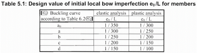
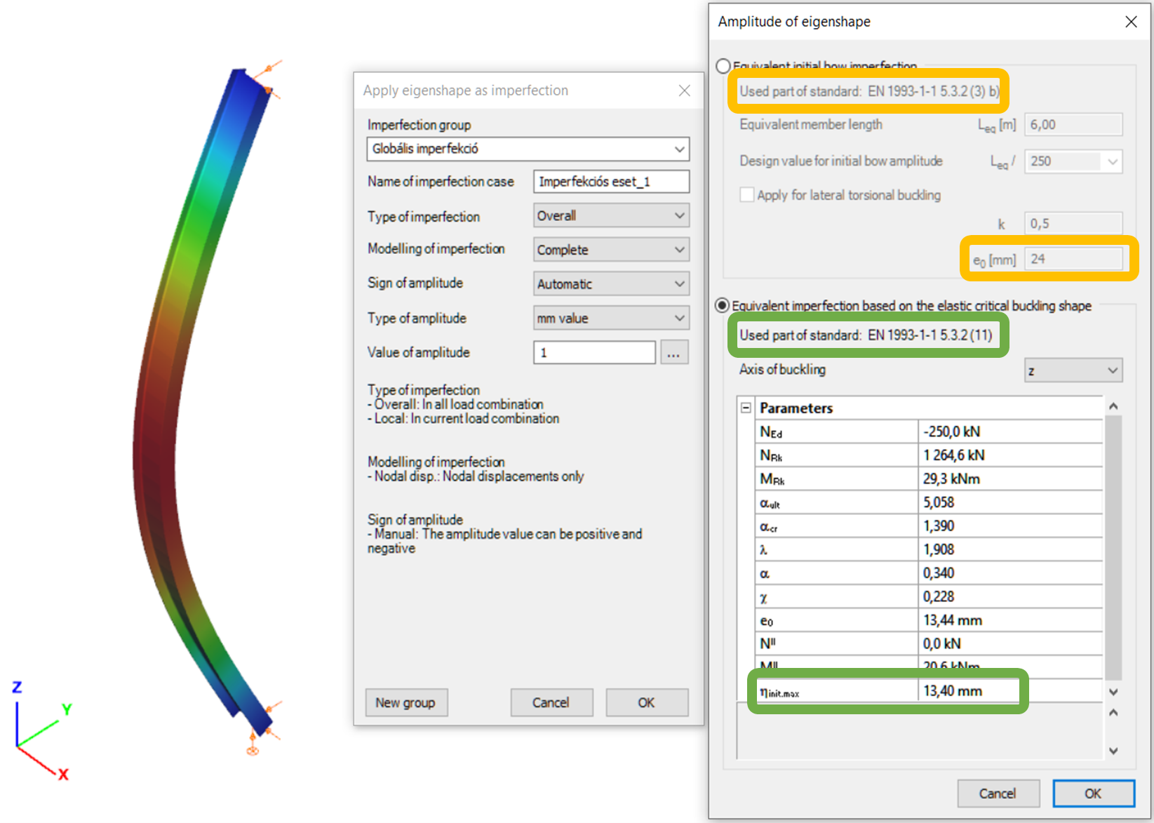
In the first part of this article, we reviewed the utilization difference and showed the relationship between the two methods. It was concluded that the method of chapters 6.3.1 (reduction factor) and 5.3.2 (11) (buckling mode based equivalent imperfection) are consistent at the load level equal to the buckling resistance of the member, so when the member utilization is 100%. The basic result of the procedure in 5.3.2 (11) is the amplitude (largest deflection value) of the equivalent geometrical imperfection. However, the Eurocode gives another simpler alternative for the calculation of this amplitude for compressed members in section 5.3.2(3) b) in Table 5.1, where the amplitude of an initial bow is defined as a portion of the member length for each buckling curves (Fig. 1.). We use the first column (“elastic analysis”) including smaller amplitude values.
It is an obvious expectation that these two standard procedures should yield at least similar results for the same problem. However, this is by far not the case in general.
In order to show the significance of the imperfection amplitudes this part is dealing with these two calculation methods, the variation of their values and the effect on the buckling utilization.
Let’s see again the simple example of Part 1: a simply supported, compressed column with a Class 2 cross-section (plastic resistance calculation allowed). The column is 6 meters high and has an IPE300 cross-section made of S235 steel. The two methods are implemented into Consteel and on Figure 2. it can be seen, that the two values for the amplitude of the geometrical imperfection is very different – e0 = 24 mm by the 5.3.2(3) b) Table 5.1 (L/250) and e0 = 13,4 mm by the 5.3.2 (11) (same as in Part 1).
Click the button bellow to download and read the full article at page 187-195.
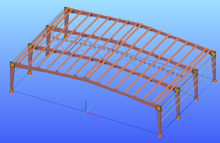
In this paper a numerical study is presented which examines a steel frame with two different finite element programs. Stability failure is more frequent in a lot of cases than strength failure hence it is important to focus on these failure modes: global, in-plane-, out-of-plane -, lateral-torsional- and local buckling. Three models were used with different elements such as shell elements and 7 DOF beam elements. 7 DOF beam elements were used in the first model, shell elements were used in the other two. The first of the shell models gave too much local buckling shapes therefore it was improved with local constraints and that is the third model where global buckling shapes can be examined. There are three different procedures to calculate the resistance: (i) the general method, (ii) the method of the reduction factors, and (iii) the simulation. The analysis results of the different programs and design methods were compared to each other and to the manual calculation based on the Eurocode 3 standards.
gateThe new versions of the EN 1993-1-1 (EC3-1-1) and the EN 1993-1-5 (EC3-1-5) standards have introduced the general method designing beam-column structures; see [1] and [2]. The design method requires 3D geometric model and finite element analysis. In a series of papers we present this general design approach. The parts of the series are the following:
- Part 1: 3D model based analysis using general beam-column FEM
Click the button bellow to download and read the full article.
gate