Is a single dominant vibration mode sufficient, or should multiple vibration modes be considered in seismic analysis?
Steel portal frames are frequently used in industrial and logistics buildings as primary load-bearing structures. Their seismic behavior is strongly influenced by the stiffness of the roof diaphragm and by the interaction between the main portal frames and secondary structural subsystems such as endwalls.
In seismic design, engineers often assume that the global response of such buildings can be represented by a single dominant vibration mode. This assumption is valid when the roof diaphragm is sufficiently rigid and the first transverse mode mobilizes most of the structural mass. However, when the diaphragm is flexible or when different structural parts participate in different vibration modes, higher modes may also contribute to the seismic response.
This article investigates how the choice between a single-mode and a multi-modal approach affects the seismic design of steel halls modeled in Consteel. Through a comparative example, the study demonstrates the implications of different modal combination techniques and discusses how reliable internal forces can be obtained while maintaining compatibility with stability verification procedures according to EN 1993-1-1.
Case with a Rigid Roof Diaphragm
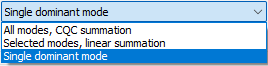
Single dominant mode
If a building is designed with a sufficiently rigid roof diaphragm, a single transverse vibration mode is typically able to mobilize close to 90% of the total participating mass. In such cases, the Single dominant mode method is an efficient and preferred design method.
A rigid roof diaphragm can be achieved by:
- Using an adequate trapezoidal steel deck, modeled in Consteel either
- as a Shear Field with a high shear stiffness parameter (“S” value), or
- by introducing equivalent dummy roof bracing diagonals with rod diameters calibrated to reproduce the diaphragm shear stiffness.
- Alternatively, real bracing elements may be added along the sidewall columns or from the eaves to the ridge along the building length.
Case without a Rigid Roof Diaphragm
If a rigid diaphragm is intentionally not assumed, a single vibration mode will generally not represent the full seismic response in the transverse direction.
Single dominant mode
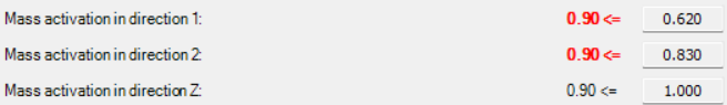
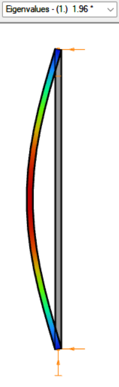
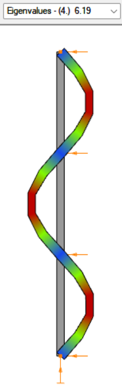
A dynamic eigenvalue analysis is first performed to determine the natural vibration modes of the structure. In Consteel, this analysis calculates the eigenfrequencies and corresponding mode shapes based on the structural stiffness and mass distribution, considering both the elastic stiffness and second-order geometric stiffness of the structure. The first three vibration modes are then evaluated for their mass participation in the transverse direction.
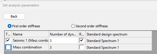
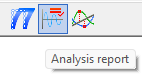
After the calculation, the mass participation for each principal direction (X, Y, and Z) can be viewed in the Analysis tab under the Analysis report, in the Mass section. In the examined case:
gateIntroduction
This article presents the calculation method for determining the buckling resistance of a pinned column with intermediate restraints in accordance with Eurocode standards. The procedure is based on an example from the Access Steel design examples collection and is compared with the calculation process implemented in Consteel’s steel member design functions, specifically within the Member Checks module.
In the following sections, a step-by-step guide is provided to demonstrate how the member check functionality can be applied to simple cases, highlighting both methodology and practical usage.
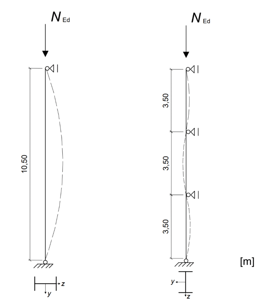
Input Data for the Example
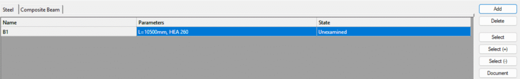
The example considers a pinned column in a multi-storey building, subjected to a design axial force of $N_{Ed}$ = 1000 kN. The column has a total length of 10.50 m and is laterally restrained about the y–y axis at intervals of 3.50 m.
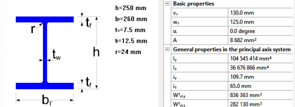
The member is a rolled HEA 260 section made of S235 steel. The cross-section is classified as Class 1. The geometric properties of the section are: height h = 250 mm, width b = 260 mm, web thickness $t_w$ = 7.5 mm, flange thickness $t_f$ = 12.5 mm, and fillet radius r = 24 mm. The cross-sectional area is A = 86.8 cm², with moments of inertia $I_y$ = 10450 cm⁴ and $I_z$ = 3668 cm⁴.
The material properties are defined according to EN 1993-1-1. Since the maximum thickness is less than 40 mm, the yield strength is taken as $I_y$ = 235 N/mm². The partial safety factors are γM0 = 1.0 and γM1 = 1.0.
Determining Design Buckling Resistance of a Compression Member
The design buckling resistance of the column $N_{b,Rd}$ is evaluated by determining the reduction factor χ for both principal buckling directions. This requires the calculation of the elastic critical forces $N_{cr}$, which form the basis for identifying the governing buckling mode.
Elastic critical force for the relevant buckling mode $N_{cr}$
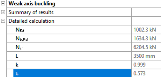
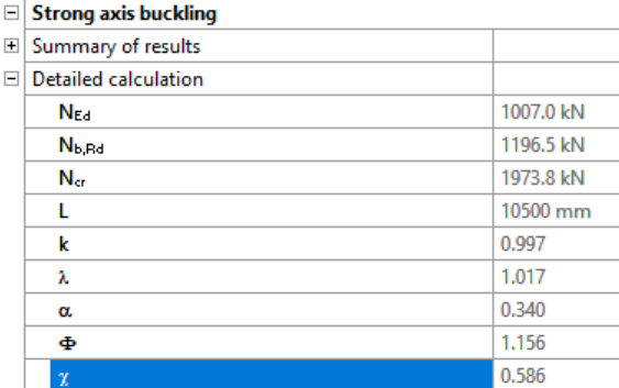
The Young’s modulus is taken as $E=210000 \frac{N}{mm^2}$. The buckling lengths in the respective planes are $L_{cr,y} = 10.50m$ for buckling about the y–y axis and $L_{cr,z} = 3.50m$ for buckling about the z–z axis. Observe that the buckling lengths for the strong and weak axes differ according to the support conditions, which must be determined by the engineer in manual calculations.
$$N_{cr,y}=\frac{π^2*E*I_{y}}{L_{cr,y^2}}=1964.5 kN$$
$$N_{cr,z}=\frac{π^2*E*I_{z}}{L_{cr,z^2}}=6206.0 kN$$
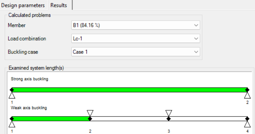
In Consteel, the elastic critical force for the relevant buckling mode can be determined using the Individual Member Design approach. This is accessible in the Member Checks tab under the Steel module, where selected members can be added and evaluated.

Once a member is selected, the analysis results are automatically loaded, provided that first- or second-order analysis results are available. Ensure that the analysis has been run in the Analysis tab and the cross section check on the Global ckecks tab before proceeding to the Member Checks section.
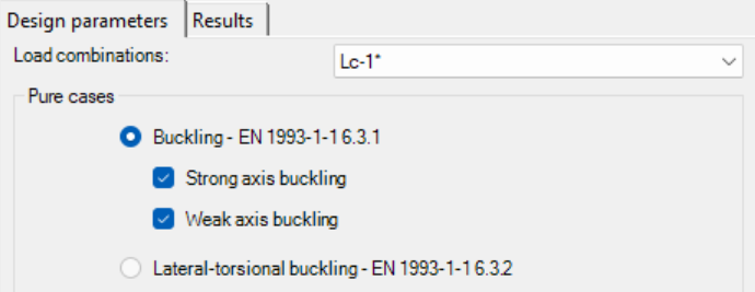
For the pinned column with intermediate restraints, the relevant buckling cases, strong and weak axis, are selected, and the dominant load combination is automatically indicated with a *. Consteel identifies the intermediate restraints separately for each direction and divides the member into segments accordingly to help determine the correct buckling lengths.
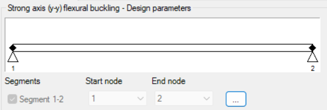
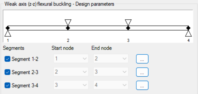
Design parameters for each segment are set with the three-dot icon:
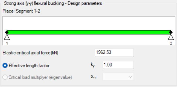
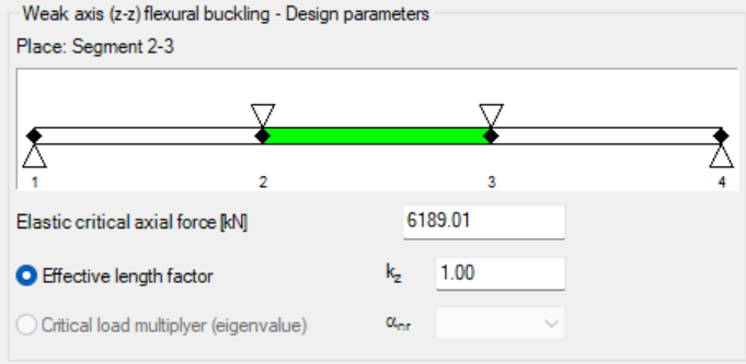
At this step, users must verify the assigned values. By default, the first value is applied, and the correct buckling shape or effective length factor should be confirmed based on engineering judgment.
In order to use the critical load multiplier selection option, make sure to perform the calculation first:


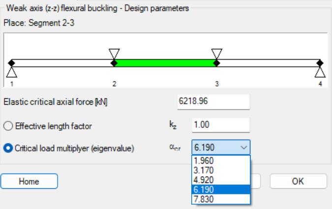
In order to check whether the correct critical load multiplier was selected, you can examine the effective length factor, which is calculated based on it (in this case, it is 1 for both directions). In our example, the relevant buckling shapes for the y–y and z–z directions are as follows:
The elastic critical force $N_{cr}$ is calculated automatically, regardless of whether the effective length factor was entered manually or the critical load multiplier was selected.
| Access Steel – manual calculation | Consteel using the effective length factor | Consteel using the critical load multiplier | |
| $N_{cr,y}$ | 1964.5 kN | 1962.53 kN | 1973.76 kN |
| $N_{cr,z}$ | 6206.0 kN | 6189.01 kN | 6218.96 kN |
Once all parameters are defined, the design check is executed by clicking the Check button, and the results are displayed.
Results can be reviewed and filtered by member, load combination, and buckling case. Lateral-torsional buckling checks follow a similar procedure, with segment boundaries adjustable and critical moments calculated either analytically or using the critical load multiplier.
Non-dimensional slenderness
In order to determine the reduction factor, the non-dimensional slenderness λ must be calculated based on the elastic critical force corresponding to the relevant buckling mode.
$$\overline{\lambda_y} = \sqrt{\frac{A*f_y}{N_{cr,y}}}=\sqrt{\frac{86.8*23.5}{1965}}=1.016$$
$$\overline{\lambda_z} = \sqrt{\frac{A*f_z}{N_{cr,z}}}=\sqrt{\frac{86.8*23.5}{6206}}=0.573$$
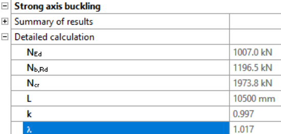
In Consteel, the detailed calculations for strong and weak axis buckling can be reviewed separately on the Results tab:
Reduction factor
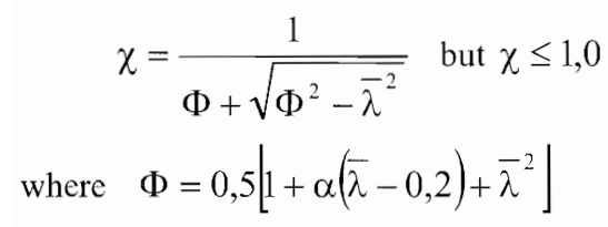
For axial compression, the value of χ corresponding to the relevant non-dimensional slenderness $\overline{\lambda}$ should be determined from the appropriate buckling curve in accordance with EN 1993-1-1 §6.3.1.2.
For $\frac{h}{b}= \frac{250mm}{260mm} = 0.96 < 1.2$ and $t_f = 12.5 mm< 100 mm$
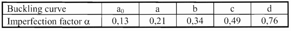
- buckling about axis y-y, buckling curve b, imperfection factor $\alpha=0.34$
$$\varphi_y=0.5*[1+0.34(1.019-0.2)+1.019^2]=1.158$$
$$\chi_y=\frac{1}{1.158+\sqrt{1.158^2-1.019^2}}=0.585$$
- buckling about axis z-z, buckling curve c, imperfection factor $\alpha=0.49$
$$\varphi_y=0.5*[1+0.49(0.573-0.2)+0.573^2]=0.756$$
$$\chi_y=\frac{1}{0.756+\sqrt{0.756^2-0.573^2}}=0.801$$
$$\chi=min(\chi_y;\chi_z)$$
$$\chi=0.585<1.00$$
Design buckling resistance of a compression member
$$N_{b,Rd}=\chi*\frac{A*f_y}{\gamma_{M1}}=0.585*\frac{86.8*23.5}{1.0}=1193 kN$$
$$\frac{N_Ed}{N_{b,Rd}}=\frac{1000}{1193}=0.84<1.00$$
Conclusion
This example demonstrates the application of the isolated member approach for a simple compression member. For more complex cases or alternative stability verification methods, such as the imperfection approach or the general method, refer to the dedicated article on stability design methods, where their principles and applications are discussed in detail.
Download modelThe latest version, Consteel 17 is officially out! In 2023, our main focus for Consteel development is improving usability. New features prioritize efficient model manipulation, easy modification, and clear information presentation across Consteel, Descript, and our cloud-based platform, Steelspace. In this comprehensive video, we walk you through a step-by-step workflow guide, demonstrating how to leverage Consteel 17 to its full potential.
If you would like to delve deeper into the new features, check out our detailed blog post for an in-depth exploration of Consteel 17’s capabilities.
Introduction
Reinforced concrete columns are essential structural elements in the construction industry. They are used, for example, in frame buildings, halls, family houses and bridges. They are used in both monolithic and prefabricated versions.
The designer aims to design safe and economical structures. As technology evolves, so do our building materials, and higher strength concrete can be produced at lower cost. As a result, the use of smaller cross-sections of columns can be advantageous.
As the columns become slenderer, stability issues and the calculation of second-order effects become more important. The ConSteel finite element program specializes in steel structures and therefore has fast and well automated solutions to stability problems.
Taking advantage of the existing features of the software, a new method for designing reinforced concrete columns, improved by ConSteel, has been made available in ConSteel version 16. It is based on the Nominal Curvature method described in Eurocode 5.8.8 [1].
To apply the Nominal Curvature Method, a lot of information is required, various material and geometric parameters. The purpose of this article is to show that the Nominal Curvature Method, as extended in ConSteel 16, answers all the questions that arise during design and is free of many of the shortcomings of the original method.
Overview of Eurocode 2 – desinging reinforced concrete columns
In this chapter, the design of reinforced concrete columns based on Eurocode 2, nominal curvature method, is presented in outline, focusing on the most important aspects.
Material parameters
Partial safety factors:
- Modulus of elasticity of concrete
?cE = 1.20 - Concrete
?c = 1.50 - Steel reinforcement
?s = 1.15
The material properties of concrete are dealt with in Eurocode 1992-1-1, Chapter 3.1.
Modulus of elasticity:
- Design value
- ?cd = ?cm/γcE
- Reducing the mean value with γcE partial safety factor
- Applicable in ULS
- In the case where creep is not considered, or considered elsewhere
- ?cd = ?cm/γcE
Creep
The calculation of the creep coefficient is discussed in EN 1992-1-1, chapter 3.1.4. Here, various factors are used to determine the final value of the creep coefficient as a function of concrete strength, using diagrams. The values can also be determined according to Annex B of EN 1992-1-1. The two calculations give almost identical results.
Imperfections
The imperfections of concrete buildings are discussed in Eurocode 1992-1-1, Chapter 5.2. It divides the imperfections into two parts. One is the global inclination, which is shown in Figure 1(b). The other part is when the network points are not displaced but the elements in between are curved. This is the initial curvature (also known as a shape error), illustrated in part c) of Figure 1.

Inclination
The effect of imperfection due to inclination can be taken into account by calculating fictitious transverse forces (nominal loads). To do this, the value of the applied inclination is calculated as follows:
- Base value of inclination
θ0 = 1/200 - Height-dependent reduction factor
αh = 2/√?
where ? is the height - reduction factor depending on the number of structural elements
αm = √0.5(1 + 1/?)
?: number of vertical structural elements bearing the total load - applied inclination
θi = θ0αhαm
Then, as shown in Figure 2, the ? the normal forces can be used to calculate the notional loads in the unbraced case: ?i = θi?.
In braced case, for example a hinged-hinged column, ?i force is not defined at the top of the column, but at the center, with the value: ?i = 2θi?.
![Isolated member with eccentric axial force or lateral force. Unbraced (left) and braced (right) - EN 1992-1-1 Figure 5.1(a) [1]](https://www.consteelsoftware.com/wp-content/uploads/2023/06/2_isolated-member-with-eccentric-axial-force-or-lateral-force.png)
Second order effects
The method described in EN 1992-1-1, chapter 5.8.8, is applicable by default to isolated columns with constant cross-section and normal forces.
The design method uses the maximum second-order moment (?2). Its distribution along the length is not directly determined. For the sake of simplicity and to be conservative, it is usual to assume this second order bending moment to be uniform along the length, but the standard also permits a sinusoidal or parabolic distribution.
If we can realistically determine the distribution of curvature, the Eurocode allows the use of the method for global structures (EN 1992-1-1 5.8.5 (3)), but this is not usually possible for manual methods due to the interactions between the elements.
To use this method, it is essential to specify the buckling length, the value of the second order bending moment depends on it. For this purpose, the standard allows the use of the factors used in the elastic theory (for cantilever ?0 = 2?, fix bottom – top hinged case ?0 = 0.7?, etc.).
Calculation of design bending moment:
?Ed = ?0Ed + ?2
where
?0Ed is the 1st order moment, including the effect of imperfections
?2 is the nominal 2nd order moment (including the effect of any curvature)
Calculation of second order bending moment from curvature
Determine the nominal curvature first:
1/? = ?r?φ1/?0
where
- ?r is a correction factor depending on axial load
- ?φ is a factor for taking account of creep
- 1/?0 is the theoretical (physical) curvature associated with failure
1/?0 = ε??/0,45?
The curvature belongs to the point where the concrete reaches its ultimate compressive strength ( ) and the tensioned reinforcement is starting to yield, i.e. the so-called “balanced” case.
The position on the design line is taken into account by the correction factor depending on axial load:
?r = (?u − ?)/(?u − ?bal)
where
- ? = ?Ed / Ac?cd
relative axial force
- ?Ed
design value of axial force
- ?Ed
- ?u=1+ω
- ω = As?yd / Ac?cd
mechanical reinforcement ratio - As
is the total area of reinforcement - Ac
is the area of concrete cross-section
- ω = As?yd / Ac?cd
- ?bal =0.4
value of n at maximum bending - (0.4 applicable in the absence of further information)
Factor for taking account of creep:
?φ = 1 + βφef ≥ 1
where
- φef = φ(∞,0) ?0Eqp / ?0Ed
effective creep
- ?0Eqp first order quasi-permanent bending moment (SLS)
- ?0Ed first order bending moment (ULS) – design combination
- ?0Eqp first order quasi-permanent bending moment (SLS)
- β=0,35 + ?ck/200−λ/150
- λ = ?0 / ?
slenderness - ?0
buckling length - i = √?c/?c
inertia radius of uncracked concrete
- λ = ?0 / ?
Second order bending moment
?2=?Ed?2
where
Second order eccentricity, where c is the factor depending on the curvature distribution. For constant cross-section ?=?2 applicable (sinusoidal distribution). In case of constant distribution ?=8 is applicable.
Design
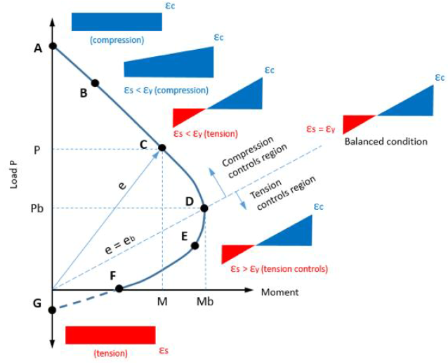
Column Interaction Curve
According to the Interaction Curve, the failure of the cross-section always occurs, when the concrete reaches its ultimate strain (usually ?cd = 0,35%).
Depending on where we are on the interaction curve, the reinforcement on the other side:
- Tensioned, and yielding,
- Tensioned, and just started yielding,
- Tensioned, but elastic,
- Compressed and elastic.
Theoretical background of the development
The design procedure is an extension of the standard procedure described in Chapter 2. It automates the manual entry of the buckling lengths and defines the distribution of the second order bending moments.
The initial value of the curvature distribution on which the calculation is based is performed on the global structure and not on an isolated column. The curvature distribution is determined from the elastic buckling shapes calculated on the whole structure (Linear Buckling Analysis – LBA).
This can be considered a realistic curvature distribution for the concrete column because we calculate the buckling shape for the entire structure, taking into account the interaction of the structural elements.
This allows the method to be extended, so that the column can now be considered not only as an isolated element, but also as part of the whole structure, in accordance with the Eurocode (EN 1992-1-1 5.8.5 (3)).
The final step, the calculation of second order bending moments (?2), is performed on an isolated model in the spirit of the standard, but for this curvature it uses the values of the corresponding buckling shape along the column calculated on the full model.
The maximum value of the buckling shape for the curvature prescribed by the standard (1/?) and the other values are varied in proportion.
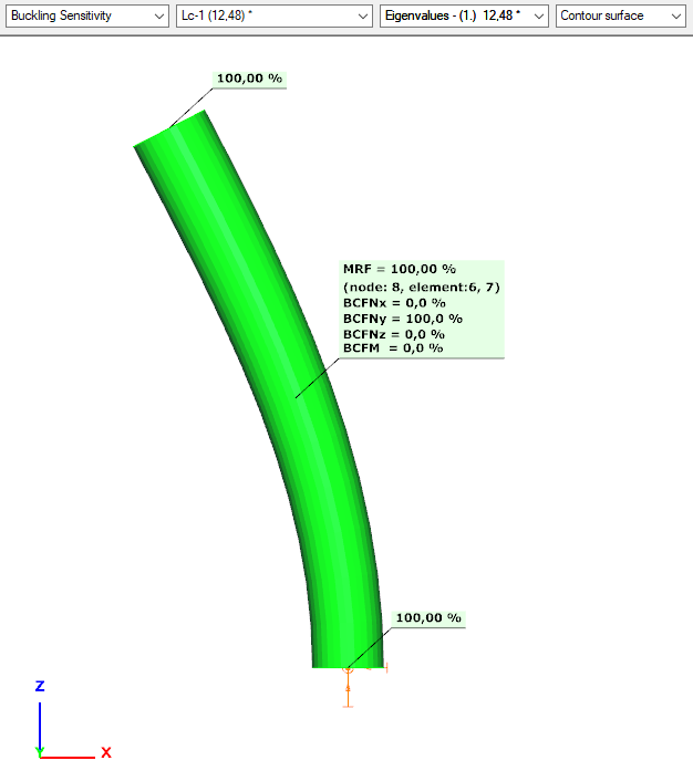
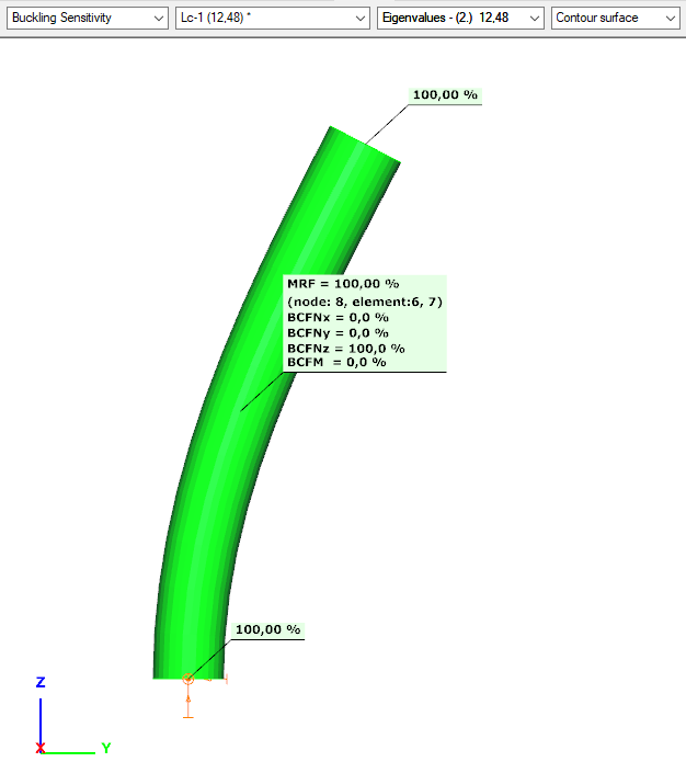
The appropriate eigenvalue assignment is done by a procedure called buckling sensitivity analysis. Magnification is performed at the point of maximum curvature found along the length of the column.
With this method, we could theoretically calculate second-order moments for any structural element and the entire structure. However, at this stage of development, it is only considered for straight-axis beam elements defined as reinforced concrete columns.
Later on, if the need arises, the procedure can be developed into a general procedure after proper testing and verification. This could be a very useful feature for example for reinforced concrete arches or reinforced concrete frame columns with moment restraints.
Buckling sensitivity analysis
The main difficulty of the method is to find the right buckling shapes for the corresponding RC columns ins both direction (x and y). The program calculates a number of buckling shapes defined by the user.
Assuming each shape as a displaced shape, the summed deformation energy per bar element is calculated along each bar element of the structure.
The element with the highest deformation energy value calculated on the basis of the buckling length just tested is assigned a value of 100%, the other elements a proportional value. The buckling shape currently under consideration is assigned to the corresponding bar element.
Since a column can generally bend in both perpendicular directions, the test is performed in both local directions and 2 eigenvalues are assigned to each column (1-1 per direction).
Calculation of second order bending moments
According to Eurocode:
?2 = ?Ed?2

where ? = π2
ConSteel calculates in a similar manner. Second order moments are calculated for each finite element of the reinforced concrete column. Three values are used. The first is the normal load at the finite element point (?Ed). The second is the second order eccentricity as defined in the Eurocode (?2).
After that, the third value is the ordinate of the buckling shape at the given finite element point, with the maximum of the buckling shape normalized to the unit value. Simply put, multiplying the first two values by this third value gives the second order moment at the given finite element point of the reinforced concrete column. This results in an improved moment distribution.
Differences compared to the standard procedure
Simplification of the calculation of the effective creep:
φef = φ(∞,?0)
conservatively, we equate the effective creep with the final value of the creep factor, without reduction. This avoids errors such as, for example, if there is no bending moment in a quasi-permanent load combination, then the value of the effective creep factor is by definition zero.
Creep factor value in ConSteel
The values given in ConSteel are taken from Table 1 of the Eurocode guide for Reinforced Concrete Structures [6].
This is based on EN 1992-1-1, chapter 3.1.4, where various factors can be used to determine the final value of the creep factor as a function of concrete strength, using diagrams.
Calculation of slenderness based on buckling analysis
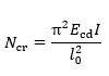
Critical strength of the Euler beam. The formula rearranged:
where
There is no need to manually enter the buckling length, the slenderness calculation is fully automated.
Second order bending moment distribution
The distribution of the second order bending moment is the same as the buckling shape, taking into account the interaction between columns.
Demonstration of the method using a console example
You can see how to make the example model in our Reinforced Concrete Column – overview article.
Download the starter model at the end of this article and open the “separate_circle_column_cantilever.csm” file.
First order analysis
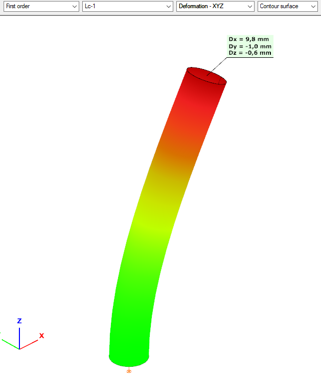
Displacement shape: realistic values:
- Slight vertical displacement
- in the direction where a greater horizontal load is applied, greater displacement
- slight displacement in the other direction due to the imperfection
- the displacement shape is curved in the direction of the horizontal load as expected
Check the internal forces:
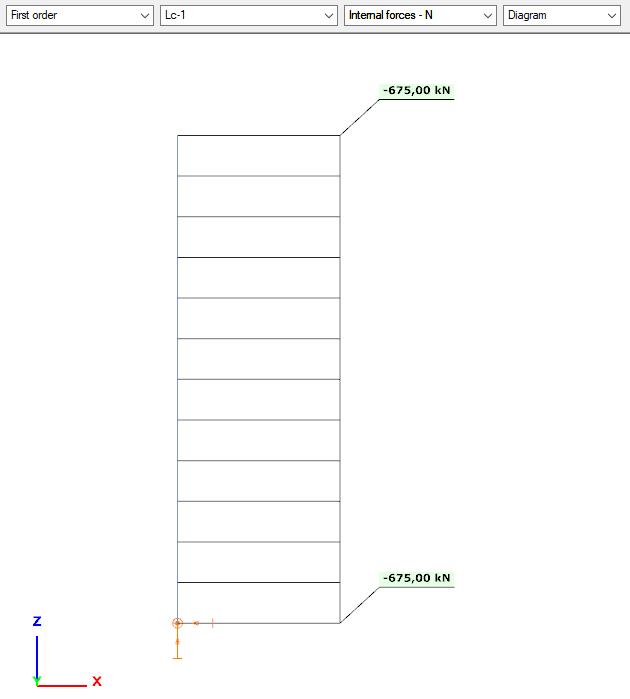
N
- same as the vertical load, with constant distribution (no self-weight applied in the model)
negative sign -> compression
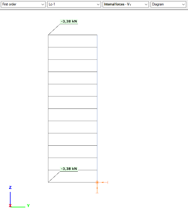
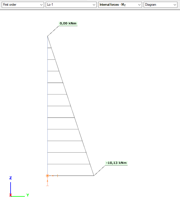
Vy+Mz
- we calculate the imperfection from the normal force
- 675*0,005 = 3,375 kN
- 3,38*3 = 10,14 kNm
- Distributions and valuer are as expected
- No Vy+Mz from applied loads, only from imperfection
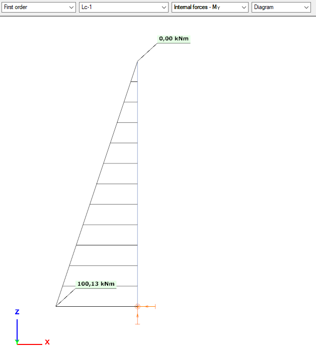
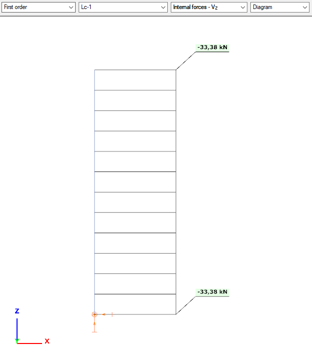
Vz +My
- Imperfection calculated form the normal force
- 675*0,005 = 3,375 kN
- 3,38*3 = 10,14 kNm
- These internal forces are calculated from imperfection
- Additional 20*1,5 = 30 kN load
- 30+3,375 = 33,375 kNm
- 33,375*3 = 100,125 kNm
- Correct internal forces
- first order internal loads from applied loads + inclination
Buckling analysis & buckling sensitivity analysis
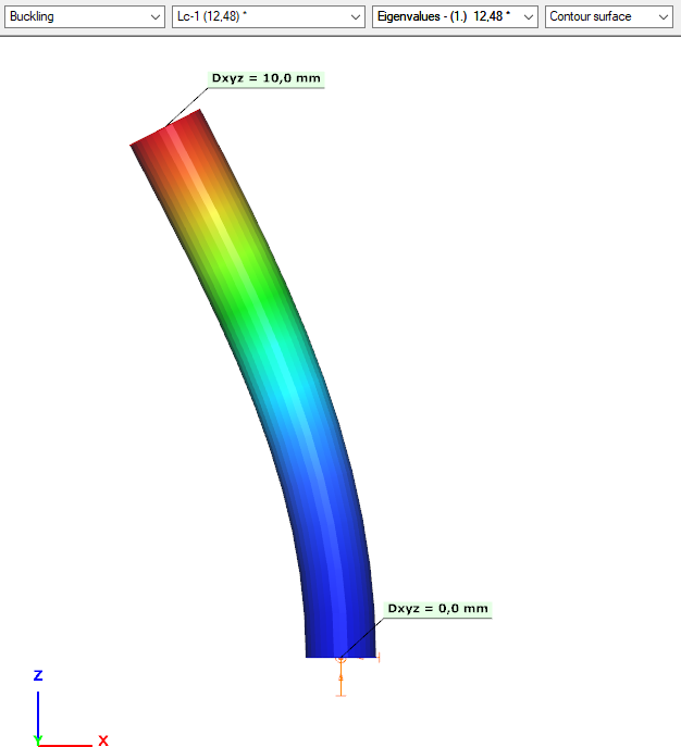
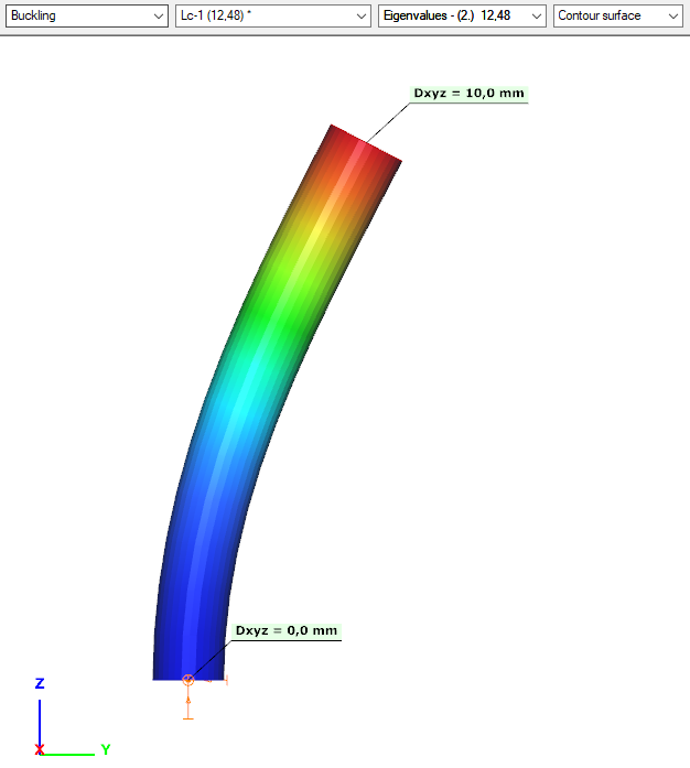
We can see from the coordinates, that this is indeed a planar buckling shape.
For a single column, it is rather easy, to check whether we have buckling shape in both directions. Here we only found one, so we need to find the other one as well.
Parameters of the buckling analysis need to be adjusted. We should increase the upper limit of the calculated number of buckling shapes.
Download the adjusted model at the end of this article and open the “separate_circle_column_cantilever_MoreBucklingShape.csm” file.
Now we have buckling shape in both x and y directions.
ULS design – EN 1992 condition
Everything is symmetrical.
GATEConsteel offers a range of load combination filtering options, which can be applied based on limit states, load cases, and analysis and design results. By applying different series of filters, designers can streamline their workflow and reduce calculation time.
Filtering options
Filtering is realized through the Load combination set definition window.
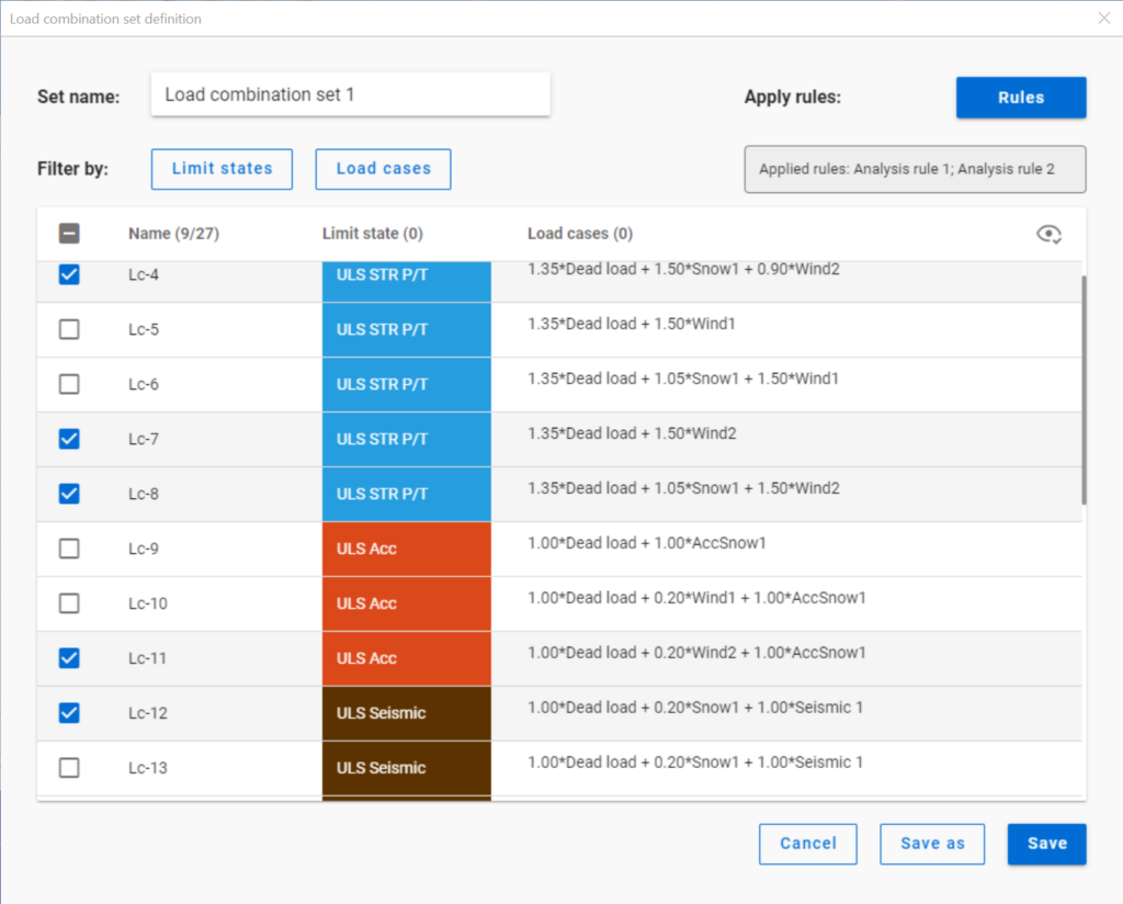
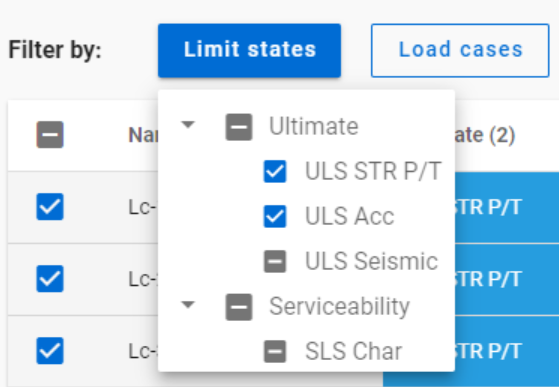
Filtering by limit states and by load cases are handled together with the checkboxes under the Limit states and Load cases buttons.
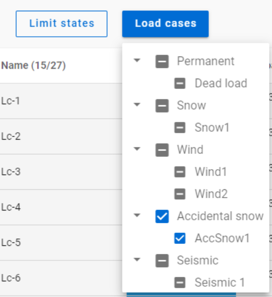
The 3-state checkboxes affect each other as they are not only used for selection but also for indication of the content. They can be manually set only to checked or unchecked. The middle state only appears when other filters are applied.
Filtering by limit states or load cases does not require any calculation results.
Filter by rules, on the other hand,is based on the actual analysis and/or design results. Different types of rules can be applied one by one or at the same time to select the desired load combinations.
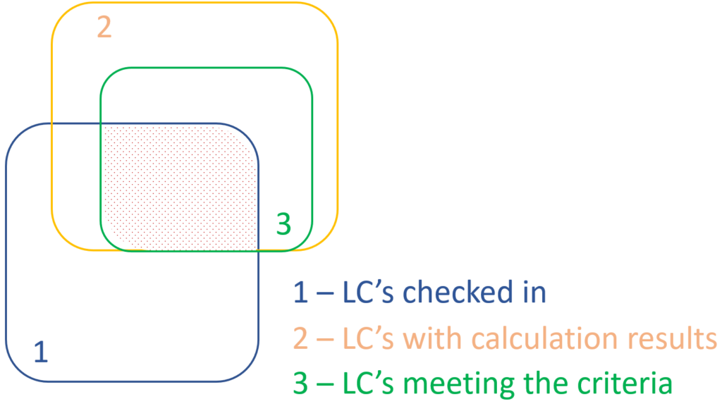
When a rule is applied, all the load combinations that are selected on the Load combination set definition dialog- either with filtering by limit states/load cases or checked in manually- are examined at every position the rule indicates. Load combinations that meet the rule’s criteria are selected (remain checked in), while those that do not, become unchecked.
- With analysis rules, load combinations can be selected based on deformations or internal forces at either every finite element node or only at the member ends. This last one is included specifically for connection design. Deformations are checked in SLS combinations, internal forces are checked in ULS combinations only.
- With buckling rules, those ULS load combinations can be selected which have the elastic critical load factor (first buckling eigenvalue) less than the given limit.
- With design rules, load combinations can be selected based on utility ratios checked in every finite element node of the chosen portion. Utilizations are available from several design checks: dominant results and detailed verifications for steel elements such as general elastic cross-section check, pure resistances, interactions and global stability. Only ULS combinations can be filtered with design rules.
Interaction of the different filter types
Filtering by limit states, load cases, and rules can be used together, with rules being applied only to load combinations that are checked in and have the necessary calculation results.
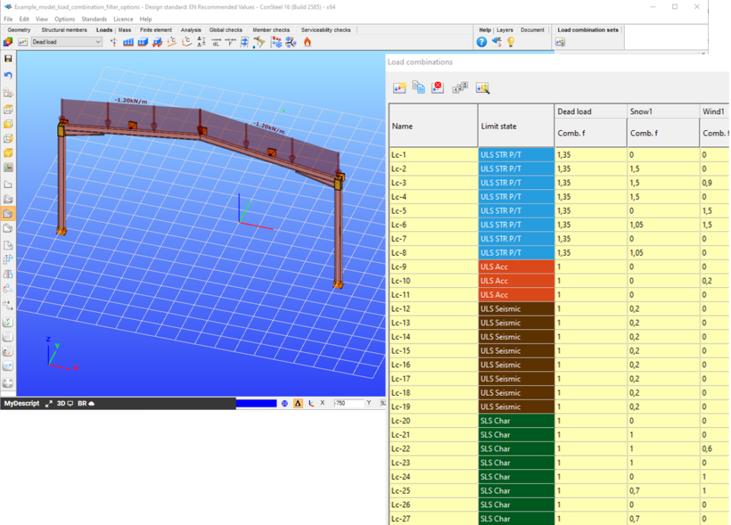
Let’s see an example.
It is a simple 2D frame model, with 27 load combinations of various limit states generated. Analysis and design results are calculated for all load combinations.
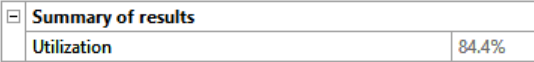
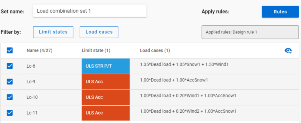
If applying design rule to select only those load combinations which result dominant utilization over 50%,

4 load combinations will be selected (Load combination set 1):
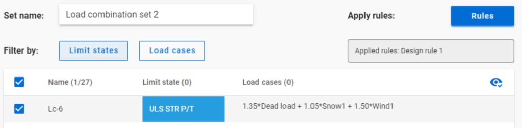
But if ULS Accidental limit state is turned off before applying the same 50% filter,
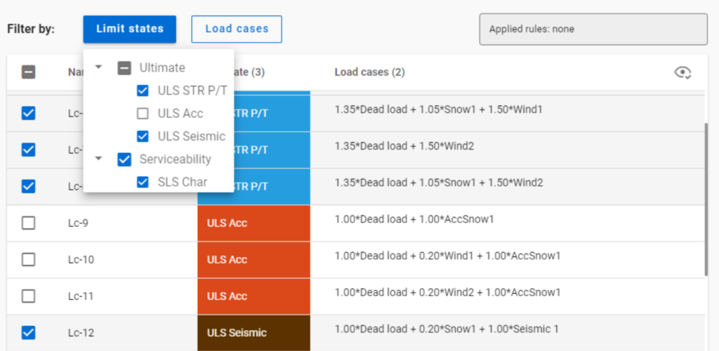
only one load combination is selected (see Load combination set 2).
Application of multiple rules
Applying multiple rules together results in the sum of the lists that would have been created separately.
gateOverall Imperfection Method in Consteel
The Overall Imperfection Method is an alternative way to carry out the buckling design for a structural member. With this method the buckling phenomenon is considered on the effect side of the equation, instead of on the resistance side, compared to the general method and the member check method. In the following video we explain the theoretical background for this calculation. After that we present application examples starting with the simplest ones, all the way to the most general case in a real-world building structure, showcasing the several extra capabilities and advantages of the Overall Imperfection Method.
Check out our user guide to learn more!
gateSmart link feature in Consteel
The smart link is a different version of the already existing link element, that was introduced into Consteel with version 14. In case of the smart link, we developed a different definition method for easier application. The smart link is also capable of updating its geometry based on changes made to other elements that it connects. This way it provides a more versatile modelling tool.
Check out the video for more info and practical examples!
gateCritical temperature calculation in Consteel
The calculation of the critical temperature is available in Consteel since the release of version 14. As an introduction of this feature, we prepared a video that gives some theoretical background on the topic, and demonstrates its usage in Consteel. It is shown how to prepare the model, how to execute the analysis and design, and how to create documentation about the critical temperature results.
Check out our user guide to learn more!
gate