
Software version: ConSteel 17 Build 3303
Keywords: Modeling; Analysis; Design; Lattice girder; Getting started;
Model examples
Design objective, choice of design standard
This design guide is intended for novice ConSteel 17 users and provides a step-by-step guide for designing a simply supported lattice girder. The geometry of the lattice girder to be designed is known from the architectural conceptual design, (Figure 1). According to the concept, the lattice girder chords are made of hot-rolled sections of HEA120, while the lattice bars are made of cold-formed SHS80x4 sections. The design of the connections is not included in this guide.

(based on conceptual design)
It is well known that structural design is always carried out according to a certain standard or its version. The selection of the standard can be made from the Design Standard menu when creating a new model in the Project Center, or it can be modified later in the Standards tab [S1] selection panel (Figure 2).
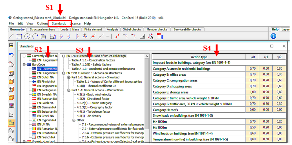
(S1: access standards; S2: select applicable standard; S3: select standard content; S4: display standard parameters).
The desired design standard can be selected from the list on the left of the panel. In this case, we select the EN Recommended option [S2]. The parameters applied by the selected standard can be accessed by selecting the corresponding row of the middle table [S3] of contents in the right-hand table [S4]. In Figure 2, the combination factors corresponding to Table 1.1 of the EC0 standard have been selected, whose parameters are shown in the right-hand table.
Setting the grid raster editor
First, let’s set the size of the raster according to the span of the structure by using the corresponding button [1] of the tool group on the left, which will bring up the Grid and Coordinate System adjustment panel (Figure 3).
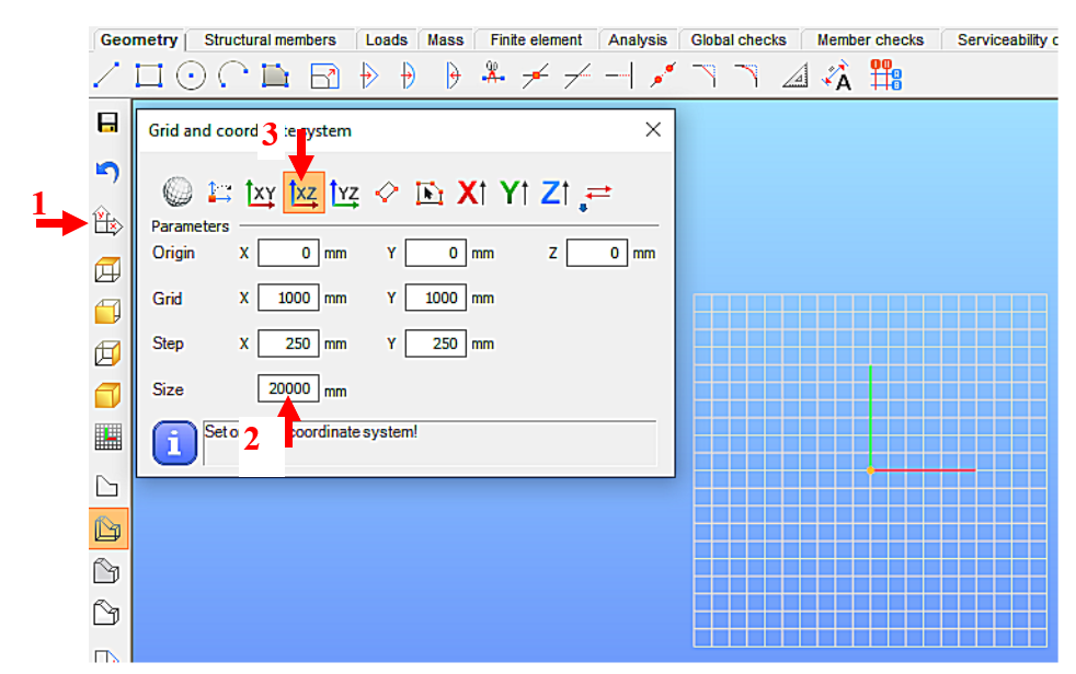
(1: set raster grid and coordinate system; 2: set raster occupancy size; 3: select view)
For example, for the 19.6m long support, the Size window can be set to 20000 millimeters [2]. To update the setting, press Enter. With the above setting, the raster will be 20m wide in X and Y directions, the raster line density will be 1000mm, and the step spacing will be 250mm. It is convenient to add the grid support model in the X-Z global coordinate plane, so the raster editor will be rotated to the X-Z plane. To do this, select the XZ plane option [3].
Loading initial cross-sections
One fundamental characteristic of general structural analysis programs is that they can only work with specifically defined cross-sections. Therefore, the first step is to choose the initial cross-sections for the task, according to the conceptual design. This may seem contradictory to the simple manual methods taught in basic statics courses, where the specific dimensions of the cross-section were often irrelevant information (e.g. calculation of internal forces). When using computer programs, however, we need to provide specific cross-sections even if their dimensions do not affect the static quantities to be calculated (e.g. in the present case, the normal forces of a truss beam). Nevertheless, we should aim to select cross-sections that match the geometrical size of the structure. In this case, the preliminary design served this purpose.
Initially, the section library for the current model is empty, so we first need to select the appropriate cross-sections. To do this, go to the Structure Members tab [4] and select the Section Administration option [5] on the left side of the horizontally positioned tool group, then select the “From Library…” button [6] in the panel that appears (Figure 4).

(4: picking up structural elements; 5: calling up the section control panel;
6: Select section type)
Figure 5 shows the loading of the HEA120 section, compliant with the European standard, which will be assigned to the chords. We select the region of the cross-section standard (European) and then its type (H profiles). From the list that appears, we can select the type of section (HEA) [7] and then the height of the section (120) [8]. By pressing the Load button [9], the program learns the cross-section, and from then on it knows everything about the cross-section and can work with it. Repeat the procedure as many times as you need different sections. Finally, the window is closed by pressing the Close button [10].
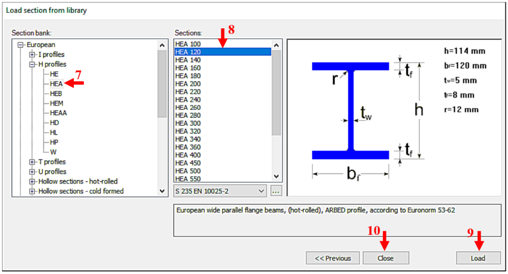
(7: select section type; 8: select section size; 9: scan selected section; 10: end loading process)
In our case, also a CF-SHS 80×4 closed section (from Library/Hollow sections – cold formed/CF-SHS/CF-SHS 80×4) was loaded for the bracing members (Figure 6).

Later on, you can obtain all the information about the cross-section using the Section module. To do this, select the cross-section in the table by clicking on the corresponding row and then click on Properties… to display all the properties of the cross-section, such as type data; cross-section characteristics, etc. The program works with two cross-section mechanical models in a dual manner. The GSS (General Solid Section) model [11] is used for static calculations and the EPS (Elastic Plate Segment) model [12] for standard design operations (Figure 7). The cross-sectional properties (surface area, moments of inertia, etc.) can be displayed by pressing the button [13].
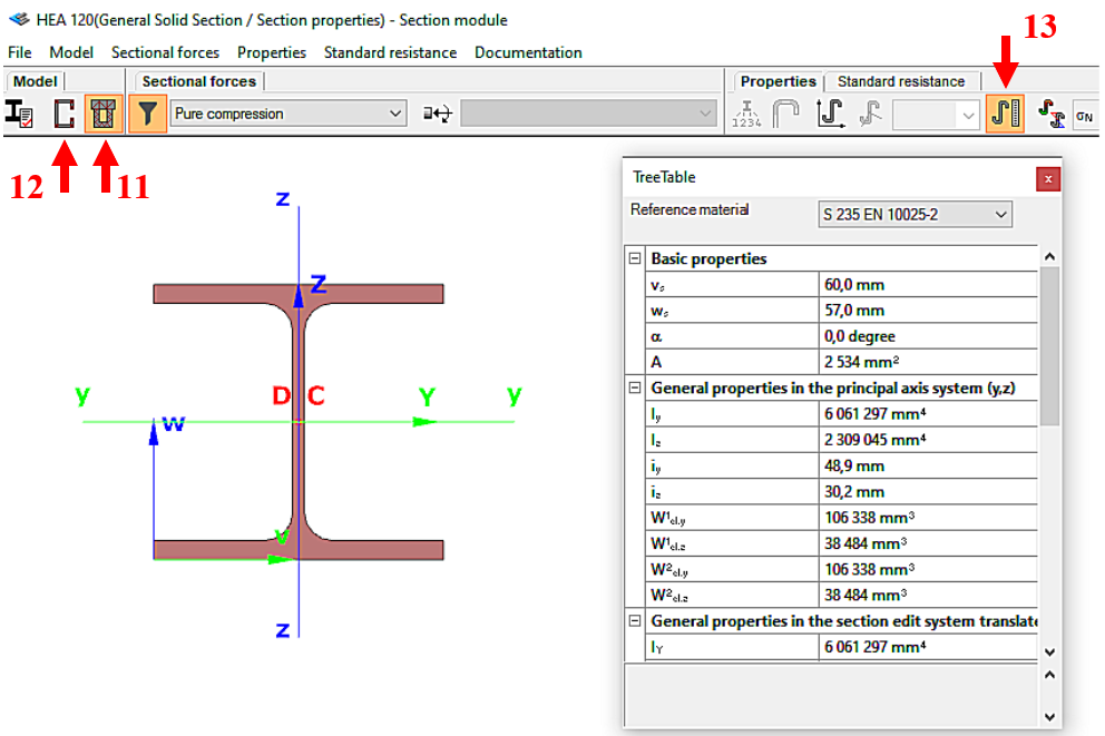
(11: Open GSS general section model; 12: Open EPS elastic plate segment model;
13: open cross-sectional properties table)
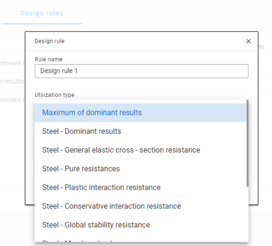
When applying design rules in load combination filter, the most frequently used utilization type is Steel – Dominant results. What results are exactly considered by this option and what do corresponding limitations mean?
Introduction
There are four ways to apply load combination filter: based on limit states and load cases, manually, and by rules. Unlike the other three methods, filter by rules is only possible based on analysis and/or design results.
The most effective way to reduce the number of load combinations is definitely the use of design rules.
With design rules, load combinations can be selected based on utility ratios. Utilizations are available from several design checks, including dominant results and detailed verifications for steel elements, such as general elastic cross-section check, pure resistances, interactions, and global stability.
The meaning of the dominant check
The dominant check is not always the check which gives the maximal ratio but the one with the maximum RELEVANT ratio. Typical example: if plastic interaction formulas are valid, those results will be dominant over general elastic cross-section check results, although the latter are higher.
Steel – Dominant results
Steel – Dominant results option contains the utility ratio of the dominant check at every finite element node, in all load combinations. Meaning that there are as many utilization values as the number of load combinations calculated, in every FE node.
It is also important to understand the difference between the utilizations of Maximum of dominant results and Steel -Dominant results. Maximum of dominant results option contains the dominant utility ratio of the dominant load combination at every node, like an envelope of Steel-Dominant results. Meaning there is only one utilization value in every FE node. Also, it is the same as the dominant result table on Global checks tab.
When a rule is applied, the utilizations of the chosen utilization type are compared against the limitation. The load combinations which give the results that correspond to the limitation, are selected by the rule. Every FE node of the selected model portion is examined.
Limitations in case of Steel – Dominant results
- Maximum: to select the combinations which cause the maximum utilization at any node. It can be the same as Maximum of dominant results, except if there are combinations where the utilization is the same and it is maximal. In this case, here all the combinations are selected, while with Maximum of dominant results, there is always one maximum.
- More than % of maximum: to select the combinations as in ’Maximum’ plus those which cause utilization that is more than the given percentage of the maximum. E.g. at a certain point max utility ratio is 80%, Limitation= More than 90% of maximum. This rule will select all the load combinations which cause utility ratios between 0,9*80=72% and 80%.
- More than: to select the combinations which cause utilization more than the defined value at any point.
Let’s see an example of a simple 2D frame for better explanation. Right-side beam is in the portion for which three design rules were applied. Five points are selected for representation but of course all the nodes of the portion are examined against the rules’ limitations.
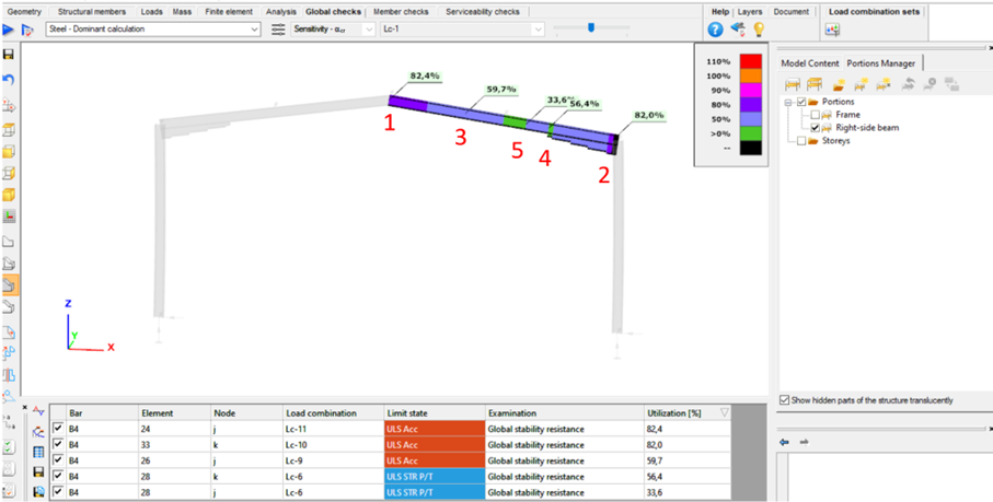
The utilizations of the five dedicated FE node in all 11 load combinations are shown on the below diagram. (To find all of these utilizations in the attached model, global checks must be calculated for the load combinations one-by-one.)
gateIn Consteel 16, we introduced the function of load combination filter. Filtering is possible based on the load combinations’ limit state, load cases, and corresponding analysis and design results. The goal is to create different sets for the different steps of the optimization and reduce calculation time while making sure that all the relevant load combinations are considered. Let’s see what a conscious design workflow looks like in practice!
Description
It is a significant problem in almost all structural design projects that the standards define many possible load cases and combinations to evaluate. Although most of these load combinations are never relevant or provide decisive design situations, it is usually not evident which ones might be neglected safely, especially when considering, that different load combinations can be relevant for different parts of the structure, like primary or secondary structure, connections, etc. Accordingly, the optimization process is overloaded by a large amount of unnecessary calculations.
With the load combination filter function, a reduced list of load combinations aka a load combination set can be created and saved for the different steps of the optimization.
The optimal workflow for the filter may vary for the different purposes the sets are created for, but there is a recommended general process that can serve as the basis for all of them. First, run the simplest calculations and use the results for a rough selection which will already decrease the number of load combinations noticeably. Then one can increase the complexity of the calculations and further reduce the list of combinations by using stricter filters. If needed, this step can be repeated. This iterative process allows us to avoid complex and time-consuming calculations for all the thousands of load combinations.
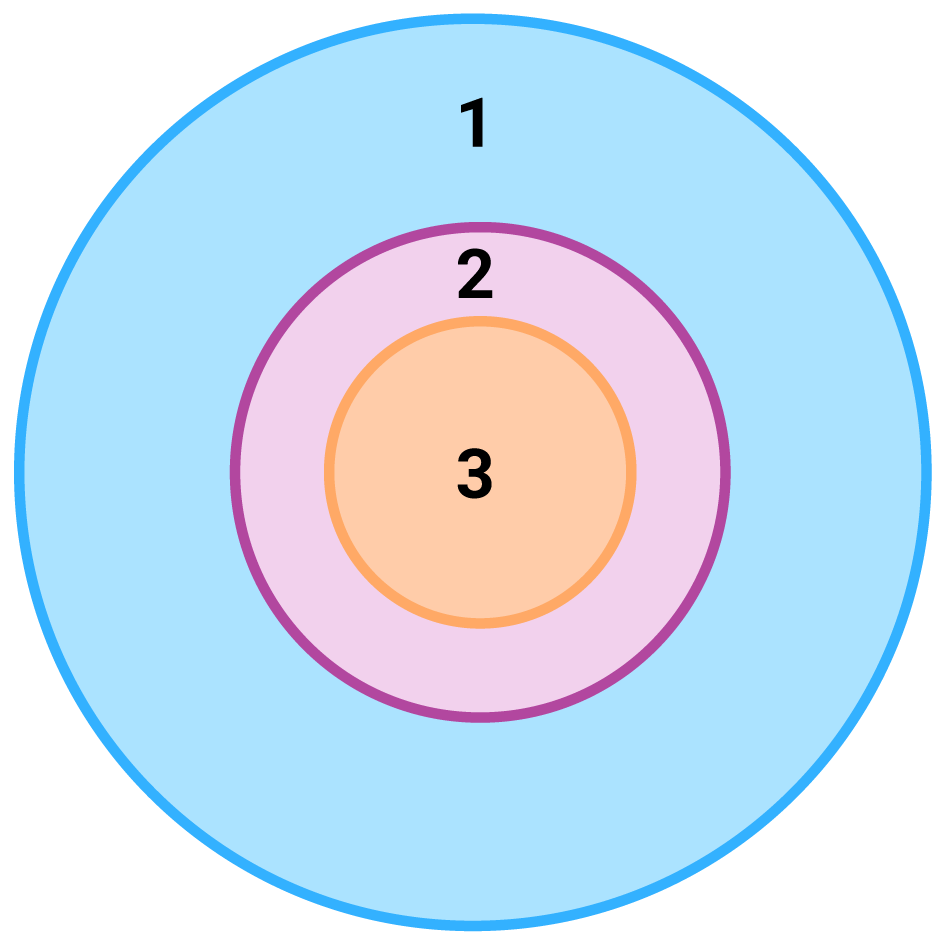
1 – all load combination, no filter;
2 – initial set with broad filter;
3 – working set with strict filter
Detailed process
Modeling
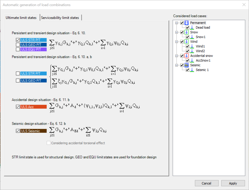
The base of all optimization processes is a correctly built structural model. So, the first step is geometrical and structural modeling and load definition. It is advisable to run a first-order analysis for only one or two load cases and diagnostics to find possible modeling errors. Load combinations can be created after that. Every limit state that will be used during the whole design of the structure, should be defined. Consteel’s automatic load combination generation function is an efficient tool to do it.
Calculation and filter
On the Load combination set definition dialog, it is possible to create load combination sets by selecting the combinations based on their limit state and/or the load cases they contain. But usually, filtering on specific analysis or design results will likely be more effective in reducing the number of combinations. Using the above-described general workflow, the steps are as follows:
gate