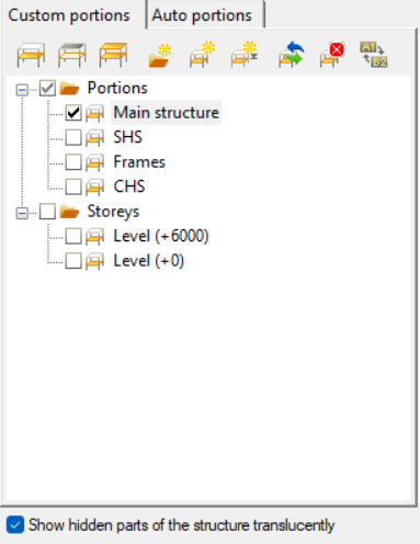
Did you know you can use Consteel to run second-order and buckling analyses on specific parts or elements of your model by defining a Custom Portion for the portion of interest?
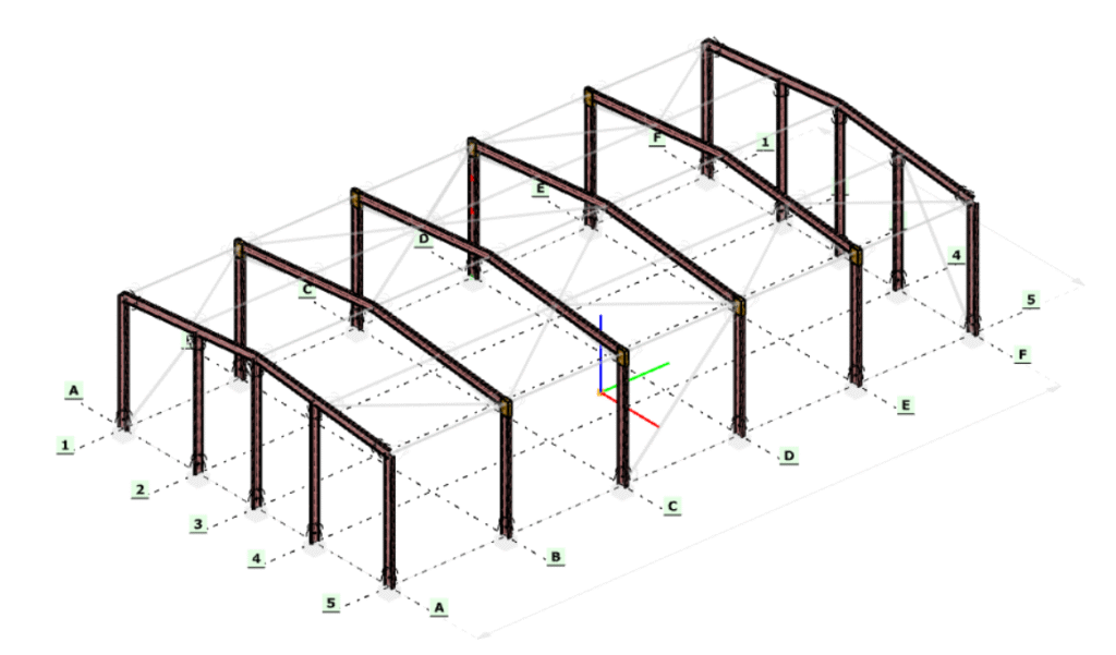
The workflow starts in the Portions Manager, where you can manually group structural members, frames, columns, beams, bracings into Custom Portions. These are fully user-defined and, importantly, only these custom portions can be directly used for analysis. This allows you to isolate exactly the structural subsystem you want to investigate, without being constrained by the full model.
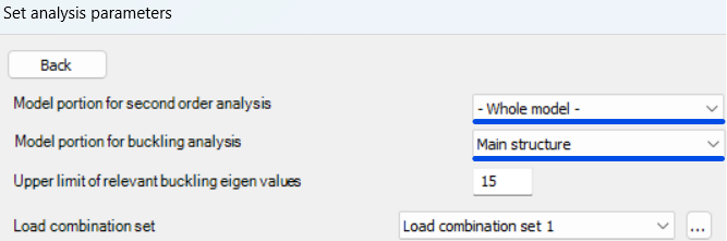
Once a portion is defined, it can be selected in the Analysis Settings, where you can choose whether second-order and buckling analyses should be performed on the entire model or only on the selected portion. The solver will then consider only that subset of elements when assembling the stiffness matrix and evaluating stability behavior.
Running these analyses on specific portions has clear engineering advantages. Second-order effects and buckling phenomena are often governed by local structural behavior, such as a critical frame, a bracing system, or a column group, rather than the entire structure. By isolating these regions, you can:
- reduce computational effort and analysis time, especially for large models
- focus on the most critical load paths and instability mechanisms
- perform faster iterations during design refinement
- avoid unnecessary influence from non-relevant parts of the structure
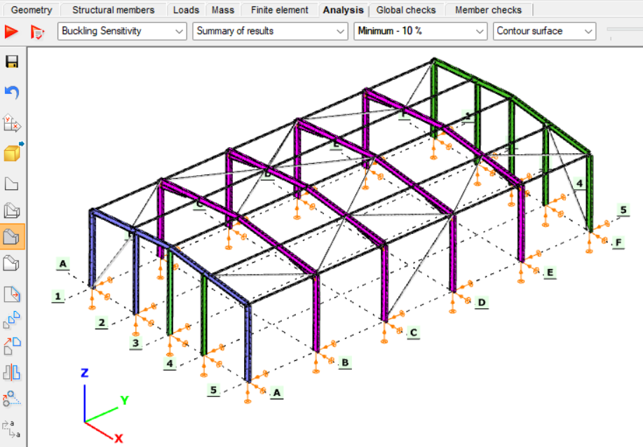
This targeted approach leads to more efficient and controlled stability analysis, particularly when investigating sensitive or highly utilized structural components.
Download the example model and try it!
Download modelIf you haven’t tried Consteel yet, request a trial for free!
Try Consteel for freeDid you know that bar members can be included in load distribution even when slightly offset from the surface, by using a Load Transfer Surface with a user-defined tolerance?
A Load transfer surface (LTS) is a special type of surface that converts surface loads into line loads and distributes them to structural members. This is particularly useful when surface loads, such as floor loads, snow loads, or wind loads, need to be transferred to supporting members.
In order to use the meteorological load generator function or our fluid-dynamics-based universal wind load generation tool, FALCON, the load transfer surfaces (LTS) on the structure must intersect, they must meet along a common edge. Otherwise, the results will not be accurate.
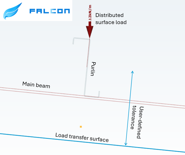
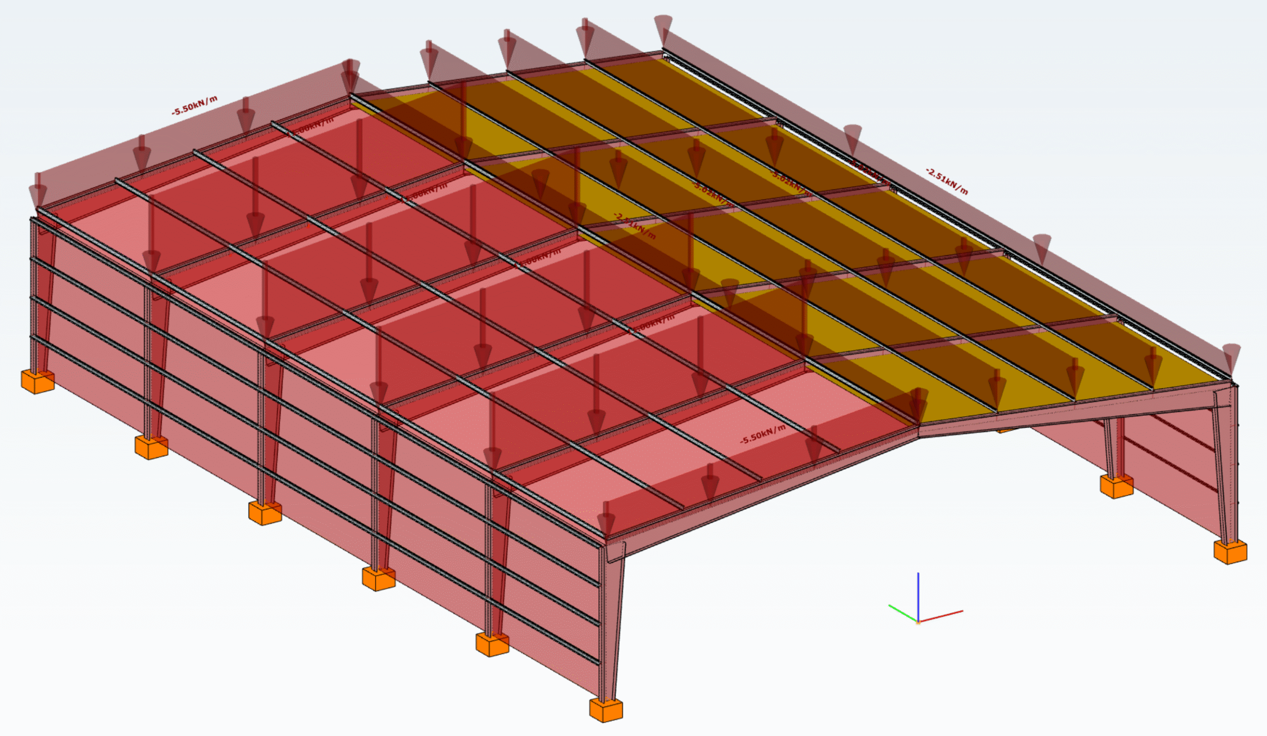
This creates a problem when, for example, the purlins take over the meteorological loads from the sheets or panels, but their planes do not intersect. In this case, the LTS is applied to the plane of the main structure, while the members assigned to it may lie within a specified distance from that plane.
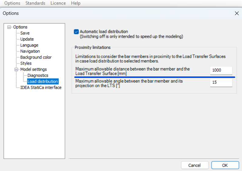
To define the tolerance for the load transfer surface, first go to the Options menu. There, you can set the maximum allowable distance between the bar members and the load transfer surface. In this example, all members that are less than 1000 mm from the surface can be assigned to the load transfer surface.
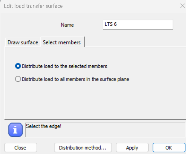
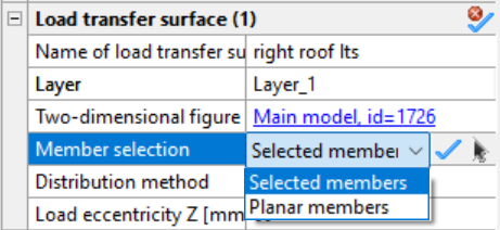
In order to be able to manually select the members attached to the load transfer surface, when defining it, make sure that in the Select members section you choose the Distribute load to the selected members option. If this option was not selected initially, you can set it later by selecting the surface and defining the member selection in the Object Properties window.
In the example model below, observe how the load distribution changes from the main beams (left side) to the tops of the purlins (right side) by introducing a user-defined tolerance and assigning the appropriate members to receive the load from the roof.
Download the example model and try it!
Download modelIf you haven’t tried Consteel yet, request a trial for free!
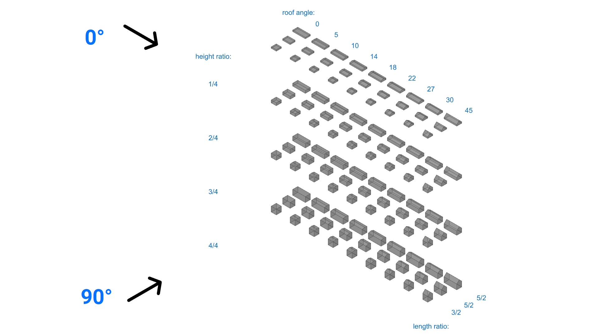
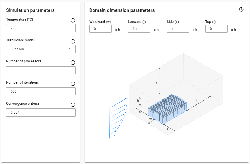
Try Consteel for freeThis study explores how Computational Fluid Dynamics (CFD)–based pressure simulation results can be compared and aligned with wind tunnel experiments and standardized design methods, reflecting the practical process engineers follow when assessing wind loads. The aim is to provide a framework for interpreting and applying simulation outputs with more confidence, supported by a clear workflow. To ensure that the findings are robust and generalizable, the analysis is grounded in a comprehensive parametric dataset: the Tokyo Polytechnic University (TPU) database of isolated low-rise buildings without eaves. This resource contains detailed pressure coefficient data for 116 building models—featuring flat, gable, and hip roofs—tested under eight wind directions, yielding more than 800 individual cases for comparison. To align these wind tunnel tests with the standard procedures the main orthogonal directions were investigated.
Compliance with standards
Before validating CFD results against established references, it is important to set the Eurocode baseline for wind load evaluation. From the wind effect side, a previous article covers how the specific wind profiles are determined and harmonized with the simulations during the preprocess phase, while for wind actions the Eurocode defines two main approaches:
- Wind pressure on surfaces – expressed through pressure coefficients for a range of building geometries.
- Wind forces on special structures – i.e. lattice towers.
Since CFD inherently produces surface pressure distributions, this study focuses exclusively on the first approach—wind pressure on surfaces—applied to closed buildings. For the purposes of this comparison, only vertical walls and simple roof types (flat and duopitched) were considered.
Under Eurocode procedures, building surfaces are subdivided into zones whose dimensions are determined by the building’s proportions. In practice, the characteristic zoning length, e , defines the extent of the regions for which local pressure coefficients are specified.
Therefore, to ensure a coherent comparison between wind tunnel tests and simulation results, the mesh refinement must be adjusted accordingly, for each previously presented geometrical case of the dataset for both principal orthogonal directions, which in turn makes a parametric study indispensable.
Parametric methodology
To support the parametric study, a dedicated script was developed to generate results for all three scenarios simultaneously: wind tunnel tests, simulation outputs, and standard-based approaches.
gateIn this article, we will explore pressure-based validation techniques applied to a simple block model within the context of wind simulation for structural engineering. Building upon our previous discussions on data processing and velocity-based validation, we aim to provide a comprehensive understanding of how pressure data can be utilized to ensure accurate and reliable wind surface loads from simulation results.
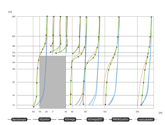
Pressure-based validation is a critical aspect of wind simulation, as it directly relates to the forces exerted on structures. During previous velocity-based validations [1] comparing the results (the average directional deviances of the velocity vector as a percentage) against established benchmarks showed that k-ε turbulence model produced the best results. Using the same simulations results the pressure-side comparison is presented below.
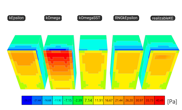
First, there is a significant difference between the simulation runtime and the iteration number, which was set to a maximum of 1000 iterations. The table below shows that the k-ε is the quickest, while k-ω SST and RNGk has not actually reached convergence. However, when comparing the global reactions calculated according to the pressure results the results are relatively close, more for the suctions on the top (Rz) and on the side walls (Ry), but less for the Rx (resulted by the pressure on the windward and the suction on the leeward walls), especially for k-ω.
Note: the Ry+ is only the resultant for one side wall of the cuboid, because the other side eliminates it, resulting a global reaction of Ry = 0 kN
| Load size [m] | 4 | ||||
| Turbulence Model | k-ε | k-ω | k-ω SST | RNGk | realizable k-ε |
| Runtime [s] | 135.295 | 392.686 | 707.589 | 663.564 | 440.801 |
| Iteration [-] | 197 | 413 | 1000 | 1000 | 342 |
| Rx [kN] | 195.63 | 315.59 | 179.88 | 176.23 | 180.22 |
| Ry+ [kN] | 94.54 | 97.75 | 92.98 | 96.95 | 95.73 |
| Rz [kN] | 53.47 | 50.02 | 52.74 | 58.64 | 54.33 |
| ADD [%] | 5.86 | 5.83 | 9.45 | 6.58 | 6.03 |
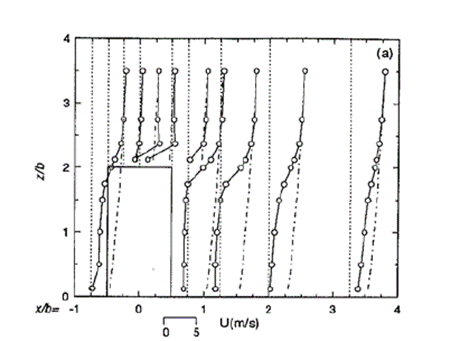
To conclude regarding the suitable turbulence models and to carry out relevant pressure-based validations it is preferable to use wind tunnel results adressing this topic directly. One of the earliest results [2] in this field by Baines, which forms the basis for the standards used today and a relatively new, thorough examination [3] by the Tokyo Polytechnic University is used as a starting point.
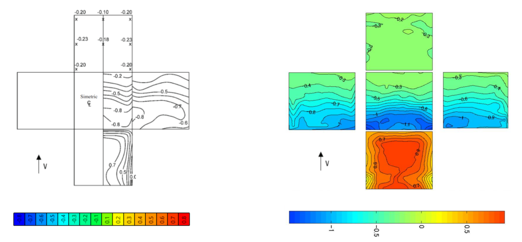
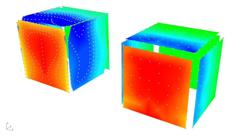
To process these results special tools were developed. The results by Baines in lack of any database was reproduced using the contour lines from the original image, while for the TPU experiment mean result values from actual measurement point results were processed in Grasshopper’s parametric environment.
Note: the color gradient for the result represenation is not harmonized according to the pressure coefficient results.
The mesh resulted by the points from the TPU results indicates an average edge length to start performing simulations. For this cuboid of 16 m x 16 m x 16 m, the ‘mesh size on the structure’ , or in other word the face edge length is 2.28 m, resulting a unified mesh suitable for post-process. For the refinement of the calculation domain a ‘mesh refinement factor’ of r = 2 was selected to reach an inlet face size below the reference height of 16 m (2.28 x 2r = 9.12 < 16). Regarding the wind profile, based on the TPU experiment, according to the Eurocode [4] a category III terrain was selected which is similar in turbulence intensity (Iv(zref) = 0.25). For the basic wind velocity, vb = 28.3 m/s was taken to produce a peak velocity pressure, qp(zref) = 1 kN/m2 for easier conversion between pressure coefficients (cpe) and surface wind loads (we).
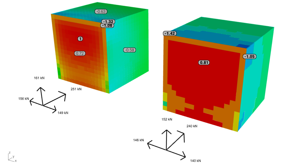
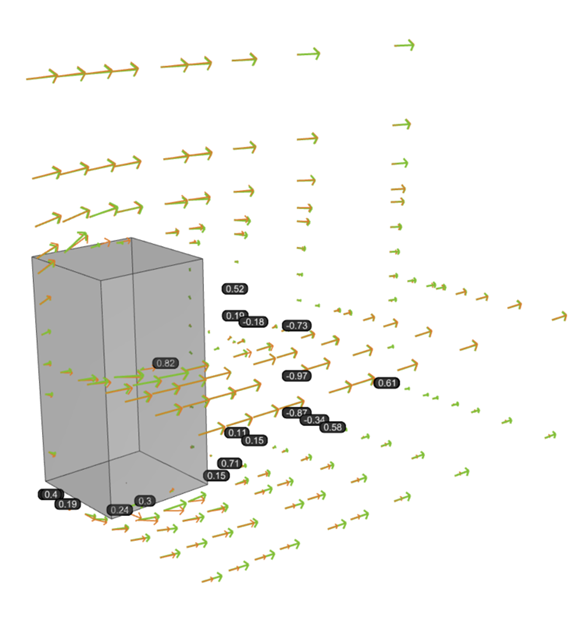
Note: the color gradient for the result represenation of all six cases below is harmonized according to the surface load results. The values with bold are the peak (min or max) values for the windward, top, and side surface, while the narrow font represents the mean value. The axis system in front is representing the resultants of the surface loads.
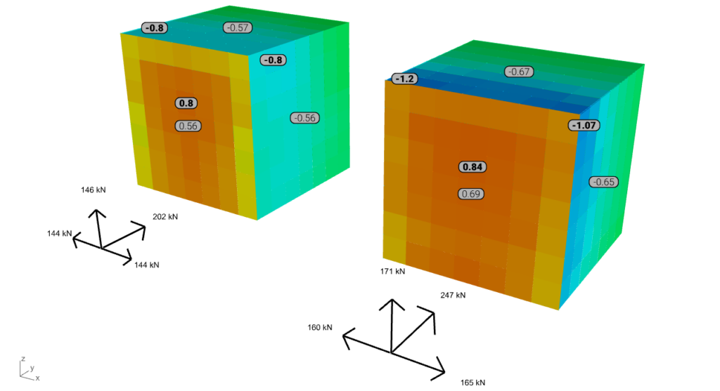
Upon projecting the experimental data onto the post-process mesh based on mesh vertex proximity, it was observed that the results from Baines are generally lower. This discrepancy is likely due to reduced accuracy at the edges and, more notably, at the corners. However, on the windward side, the maximum pressure coefficient is approximately 0.8, while the suction values also align with typical Eurocode values.
When examining global reactions or resultants, the simulation outcomes tend to align with the TPU results, especially on the windward side. Conversely, for the suctioned surfaces, such as the side walls and top, the simulation results are generally lower on average.
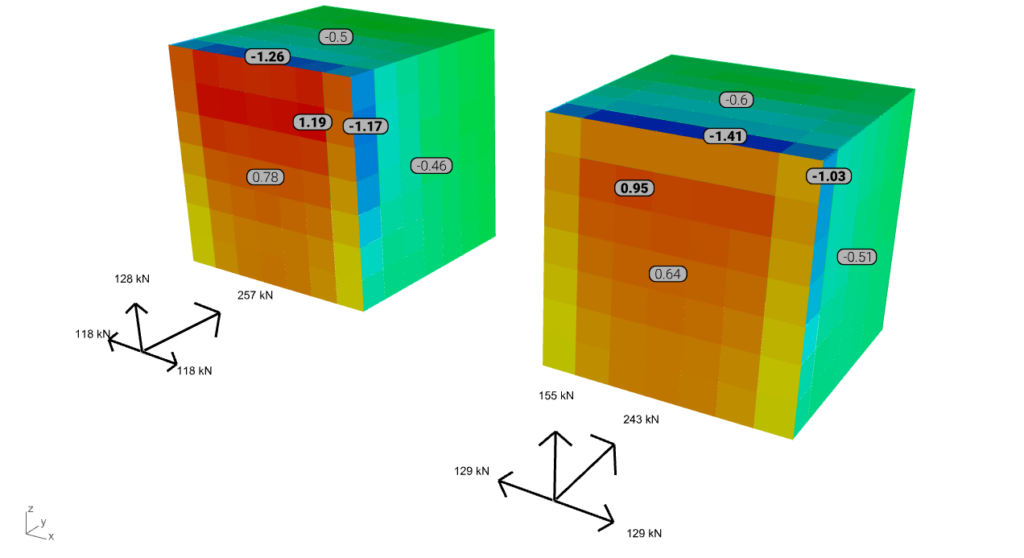
From the perspective of this pressure-based validation k-ω SST demonstrates improved accuracy, particularly when the ‘mesh size on the structure’ is refined to 1 meter. This refinement enhances the correlation of results, including on the suction sides. However, the model’s robustness can be questionable, leading to increased computational time for convergence.
For structural engineering purposes the zoning of these loads can actually offer efficiently usable loads during structural analysis, comparable with standards. From this scenario two advantages of simulated loads can already be observed:
- For the windward side loads with similar distribution to the wind tunnel experiment can be produced, leading to reduced loads instead of one uniformly distributed surface load (D zone of Eurocode)
- For the side walls the decrease of the loads along the height can also be produced with simulation, leading to reduced load areas for A zones of Eurocode
While obtaining wind tunnel experiment data for thorough, double-checked validation can be challenging due to limited background information, our current validations already highlight that mesh density and the appropriate selection of turbulence models are pivotal factors significantly affecting pressure distribution. Striking an optimal balance between accuracy and computational efficiency remains the challenge of the beta testing period. Consequently, in forthcoming articles, we plan to broaden our validations to encompass larger-scale models with typical geometries. This expansion aims to facilitate meaningful comparisons with established standards and to provide comprehensive guidelines for efficient wind load generation post-processed from simulation results.
References:
[1] Dataprocessing and velocity-based validation on a simple block – https://consteelsoftware.com/ro/knowledgebase/dataprocessing-and-velocity-based-validation-on-a-simple-block/
[2] Baines, W. D., 1963. Effects of velocity distributions on wind loads and flow patterns on buildings, Proceedings, International Conference on Wind Effects on Buildings and Structures, Teddington, U.K., 26–28 June, 198–225
[3] Aerodynamic database for low-rise buildings – https://wind.arch.t-kougei.ac.jp/system/eng/contents/code/tpu
[4] EN 1991-1-4: Eurocode 1: Actions on structures – Part 1-4: General actions – Wind actions
In this second article of our wind simulation series, we will delve into two critical topics of wind simulation for structural engineering. The first one is data processing, a collective name for the most relevant steps of the fluid-dynamics aided wind load generation, such as mesh creation, executing the simulation itself and extracting initial results. While the second one is a preliminary velocity-based validation example to broadly explain the influence of the simulation parameters, to ensure that the results are accurate and useful for practical design applications.
In the previous article [1], we covered the preprocessing steps for wind simulation, including setting up the geometry using simulation surfaces and boundary conditions (wind effects and directions). These parameters were mostly aligned with the underlying logic of the standards, therefore their interpretation is relatively straightforward. However, to carry on it is inevitable to briefly introduce the simulation related parameters too, which are divided into two categories.
The basic settings are the ‘mesh size on structure’ and the ‘mesh refinement factor’. The first one is the average edge size on the structure for both of the generated meshes, the finite element mesh for mechanical and the the finite volume mesh for fluid-dynamical purposes, presented in the previous article. While the refinement factor is used to increase the finite volume cell edge sizes at the boundaries of the simulation domain, which are considered to be far enough from the building, therefore it is not necessary to calculate field values as densely as it is calculated around the building according to the ‘mesh size on structure’ parameter, leading to quicker simulations.
Note: Larger mesh size on the structure and larger refinement factor values are leading to coarser mesh, therefore a quicker simulation but less accurate results!
The advanced settings are a set of parameters to control the simulation in the background, with default values usually leading to adequate results. However the goal of this article is to provide an insight in their influence.
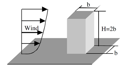
To ensure a meaningful validation, a wind tunnel test was replicated, utilizing experimental data and computational parameters from the Architectural Institute of Japan (AIJ) Benchmarks [2] . The experiment was carried out in a small circulatory wind tunnel at the Technical Research Institute of Shimizu Corporation. The test model consisted of an acrylic cuboid with dimensions of 160 mm in height and 80 mm in width. The inflow wind velocity was set at 6.75 m/s, with a measured turbulence intensity of approximately 0.5%.
Note: These validations were performed in a development version of our tool in the Grasshopper enviroment. In Consteel the tool focuses on the generation of wind loads, therefore can be utilized to extract pressure values.
Several key aspects were considered throughout the entire analysis process of the case study. Given that the model represents one of the simplest geometries encountered in practice, and that its structural behavior is straightforward to interpret within the context of standard guidelines, this case served multiple purposes. Primarily, it was used to underline the importance of conducting mesh independency tests prior to the actual simulation. As indicated in the table below, even for a simple geometry, the influence of mesh density proved to be significant — not only in terms of result accuracy but also from a performance perspective. For further investigations the “2000-4” mesh configurations was chosen, where the convergence of results became apparent.
| Mesh size on structure [m] | 8000 | 4000 | 2000 | 1000 |
| Mesh refinement factor | 2 | 3 | 4 | 5 |
| Meshing runtime [s] | 18.3 | 65.3 | 61.2 | 108.9 |
| Cell number [-] | 136432 | 150881 | 264786 | 495694 |
| Simulation runtime [s] | 65.3 | 57.9 | 151.1 | 343.4 |
| Iterations [-] | 264 | 182 | 260 | 314 |
| Fx+ [kN] | 197 | 203.0 | 205.6 | 203.5 |
| Fy+ [kN] | 94.4 | 94.5 | 89.9 | 89.7 |
| Fy- [kN] | 94.5 | 94.4 | 89.8 | 89.8 |
| Fz+ [kN] | 53.6 | 52.4 | 47.7 | 48.2 |
The next aspect was to emphasize the significance of mesh refinement, particularly along the edges. For example, finer mesh resolutions capture higher suction values on the side walls, though over smaller localized areas. Consequently, it is crucial to closely monitor the global reactions from the acting pressures influenced by a given mesh configuration, as presented in the table above.
Following the initial calibration tests, five different turbulence models (k – ε, k – ω, k – ω SST, RNG k – ε, Realizable k – ε) were compared based on their respective velocity fields.
These cases were executed simultaneously to assess the impact of full processor utilization. During the meshing process, the same mesh was applied in nearly all cases; however, the runtime increased to approximately 250 seconds, which is four times longer than when the cases were run separately. This clearly indicates that the previously reported runtimes were significantly influenced by the concurrent execution of parallel processes.
Note: It is also possible to run a single simulation case in parallel, which involves decomposing the computational domain and subsequently reconstructing it. However, this decomposition process also requires computational resources, meaning that running simulations in parallel does not always result in faster execution times.
The primary metric used for each case was the average directional deviance of the velocity vectors obtained by simulation from the benchmark experiment velocity vector, where 0 indicates parallel vectors and 1 indicates perpendicular vectors. Across all scenarios, similar behavior was observed in the wake region of the building, underlining a key limitation of RANS-type turbulence models. Specifically, these models tend to capture only a single dominant vortex during flow separation, resulting in the highest deviations behind the building, as well as near the ground.
To assure relevant and transparent validations the original AIJ benchmark results were compared with the results obtained using several turburent models in a similar manner. A set of points close to the building inside of the calculation domain were monitorized.
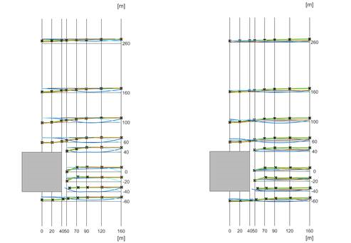
In conclusion, while these validations based on velocity fields may have limited direct relevance from a structural engineering perspective, understanding the flow behavior around buildings and calibrating simulations appropriately remains crucial. It is evident that even for simple geometries, simulation results are highly sensitive to parameter variations, underlining the need for an iterative approach to ensure mesh independence and result convergence.
During the investigation, the objective was to establish a general guideline for better starting values. As such, a mesh size on structure between e/12 and e/20 is recommended for the structure, where “e” corresponds to the minimum value between the crosswind width of the structure and twice its height, as defined in EC 1991-1-4 [3]. Using this as a starting point, it is advisable to apply an iterative simulation process with a refinement factor ranging from 5 to 0, while continuously monitoring the convergence of pressure results. This iterative method forms the foundation of the load generation procedure during the post-processing phase, which will be further discussed in upcoming knowledge base materials.
References:
[1] Preprocessing wind simulation for structural engineering purposes
[2] Guidebook for CFD Predictions of Urban Wind Environment – Architectural Institute of Japan
[3] EN 1991-1-4: Eurocode 1: Actions on structures – Part 1-4: General actions – Wind actions
As we prepare to publish the first version of our wind simulation tool, let’s explore the theoretical and technological background that makes it unique. Throughout the development process, we identified a significant gap between computational fluid dynamics and structural mechanics, highlighting a substantial amount of knowledge that needs to be bridged. With our commitment to fostering a responsible developer-user community, we’ve decided to release several knowledge base materials in the upcoming months to explain the key features that primarily will operate behind the scenes within the Consteel design workflow. The first step is to understand the prerequisites of the tool and how we aim to align the finite element, standard-based approach of structural engineering with the finite volume methods used in computational fluid dynamics. In short, we refer to this as preprocessing. So, let’s delve into what that entails.
In structural engineering, the evaluation of wind-induced loads is typically carried out using standard procedures designed to simplify the process in various ways. However, when more advanced methodologies like computational fluid dynamics are utilized, these standards inevitably serve as a benchmark, providing a basis for comparison against the pressure results generated by the simulation.
The entire development process was centered around determining wind profiles using standard procedures. The first implementation follows Eurocode 1-4, which is based on a set of parameters, organized similarly to the Consteel interface for defining meteorological effects.
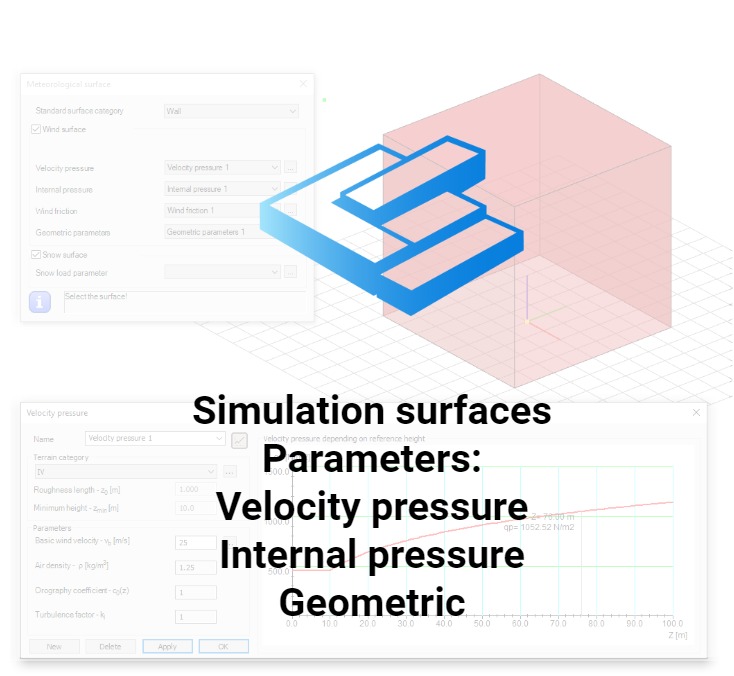
The velocity pressure parameters include the basic wind velocity (vb), which can be selected based on geographical zones specific to each country, and the terrain category. The terrain category, as defined in a selected national annex, provides values for roughness length (z0), minimum height (zmin), and the terrain factor (kr). The terrain factor can either be a fixed value, as specified in several national annexes, or calculated using a proposed formula based on the roughness length and minimum height. Additionally, the selected national annex provides essential values for air density (ρ), orography coefficient (co(z)), and turbulence factor (kI), among others.
Internal pressure parameters include coefficients that modify the velocity pressures for a given wind direction, replicating the effects of internal pressures as described in the Eurocode.
Note: At this stage of development, we strongly recommend using the tool solely for achieving external pressure on closed, ‘air-tight’ buildings.
The geometric parameters include the basic wind direction definition according to the global coordinate system (θ = 0°), the ground level (Z), and other dimensional parameters. These parameters can be used to create zoned loads, allowing for load contours similar to those defined in the Eurocode.
Finally, simulation surfaces are the surfaces enclosing the investigated building. acting as load transfer surfaces for subsequent mechanical calculations.
Note: Currently, simulations are limited to surfaces and cannot be performed on beam members.
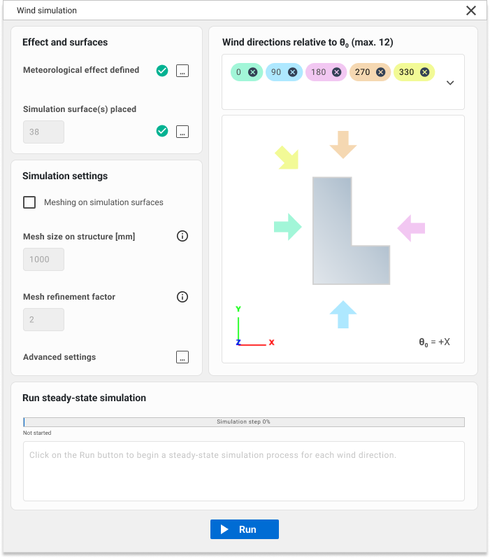
Once all the necessary parameters which are aligned with the underlying logic of the standards are collected, the actual preprocessing can be initiated from a separate dialog. This interface requires additional CFD-related inputs, which will be explained in the upcoming knowledge base materials.
The preprocessor can be observed as an operational phase or a collection of methods, with two primary tasks executed based on the previously gathered parameters. The first task is to convert the input geometry into a specially developed mesh format (FoamMesh). This format resembles a traditional finite element mesh, featuring triangular or quadrilateral planar faces and vertices, and is capable of storing simulation results. Additionally, FoamMesh can interpret meshes with polygonal faces (‘Ngons’), typically generated by OPENFOAM®, which can often be non-planar. Besides, faces can also form zones based on their results. For representation purposes, these meshes can be viewed as a list of polylines (or two-dimensional figures in Consteel) at any time.
Note: The finite element mesh used for simulation differs from the mesh employed for load distribution in mechanical calculations. The internal vertices of this simulation-specific are obtained through the iterative offset of the surface contour, aiming to primarily create quadrilateral faces. These quad faces are preferred for zoned load creation during the postprocessing phase.
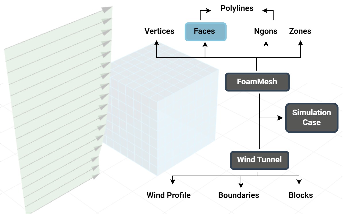
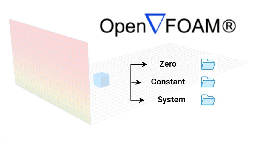
The other task is to generate a virtual wind tunnel, which consist of the wind profile according to the parameters, and the actual closed domain in which the simulation is performed defined by boundaries and inner blocks (finite volumes). Having these two it is possible to create the simulation case contents proper to the OPENFOAM® hierarchy. The wind flow parameters are stored in ‘zero’ folder, mesh generation both in ‘constant’ and ‘system’, while solution and result query parameters in ‘system’.
Note: For each wind direction a separate simulation case is performed, with it’s own independent finite volume mesh based wind tunnel. However, the finite element mesh of the building is identical, regardless the direction.
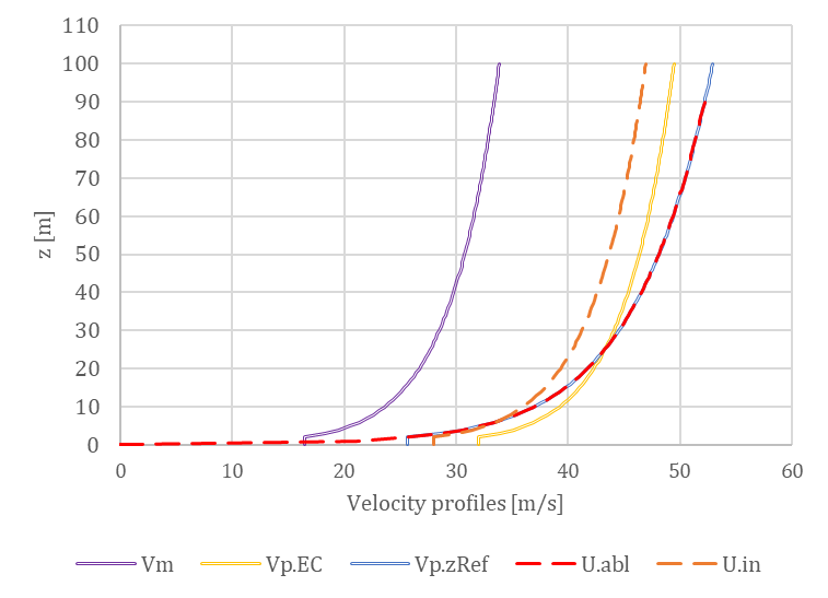
Regarding the wind profile, the clear objective is to introduce a wind velocity profile that replicates the peak pressure profile specified by the code. However, defining this profile is not straightforward. The figures below illustrates various approaches, with the QpEC function representing the general ‘target’ profile according to Eurocode.
Since Eurocode typically neglects the second-order term of turbulence intensity (considering only 1 + 7Iv(z)) when calculating QpEC, a significant difference arises if we calculate the velocity pressure, QpEC.V, from the peak velocity profile (using 1 + 3.5Iv(z) for turbulence intensity). As a result, VpEC is not intended to be directly implemented in OPENFOAM®.
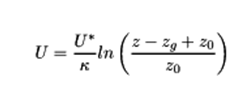
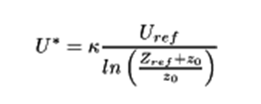
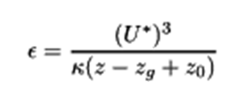
Besides the standards, OPENFOAM® offers a default approach for logarithmic atmospheric boundary layers (Uabl), based on the friction velocity U* calculated at a reference height. However, the resulting Qp.abl also shows a significant difference, lacking the constant segment below the minimum height (zmin). Otherwise, this profile is similar to a standard Vp(zRef), which is evaluated along the height using only one exact turbulence intensity value calculated at the reference height (Iv(zref)).
The logarithmic profile evaluated by the atmospheric boundary layer approach of the OPENFOAM® is according to the followings:
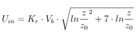
Therefore, it was necessary to develop a unique solution within OPENFOAM® for the determination of the Uin as the inlet peak velocity profile, which produces the desired QpEC. This uses the following formula:
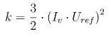
For an inlet wind profile using the k-ε turbulence model the initialization of the k and ε field values is also necessary. For this, there are also different approaches to consider. The basic atmospheric boundary layer of OPENFOAM® calculates a constant value along the height automatically, according to:

However, the inlet turbulent kinetic energy is generally calculated based on the inlet reference velocity and the turbulence intensity, which is defined by Eurocode according to the terrain parameters as presented previously:
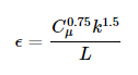
Similarly for the inlet ε there is a default automatic way used by the OpenFOAM based on the friction velocity:
And there is also an approach considering the turbulent length intensity which can be evaluated according to a Eurocode procedure:
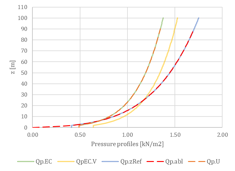
These approaches were compared for both the mean velocity and the peak velocity profiles, as shown in the figure below. The peak pressures correspond to the values measured on the windward wall of a simple 8 m x 8 m x 8 m cuboid. The naming conventions for the profiles are as follows: inlet velocity profile (mean and peak) – inlet turbulent kinetic energy (automatic – a or calculated – c) – inlet turbulent dissipation rate (automatic – a or calculated – c).
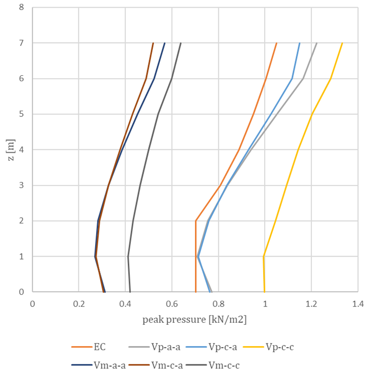
In conclusion, the profile chosen for implementation is the Uin, with automatic evaluation applied to both the inlet turbulent kinetic energy (k) and the inlet turbulent dissipation rate (ε). The effects of various turbulence models, along with the influence of different meshing procedures on the geometry, to which we refer as dataprocessing, will be discussed in upcoming knowledge base materials. So stay tuned as we explore different validations of this newly developed tool.
Software version: ConSteel 17 Build 3303
Keywords: Modeling; Analysis; Design; Lattice girder; Getting started;
Model examples
Design objective, choice of design standard
This design guide is intended for novice ConSteel 17 users and provides a step-by-step guide for designing a simply supported lattice girder. The geometry of the lattice girder to be designed is known from the architectural conceptual design, (Figure 1). According to the concept, the lattice girder chords are made of hot-rolled sections of HEA120, while the lattice bars are made of cold-formed SHS80x4 sections. The design of the connections is not included in this guide.
")
(based on conceptual design)
It is well known that structural design is always carried out according to a certain standard or its version. The selection of the standard can be made from the Design Standard menu when creating a new model in the Project Center, or it can be modified later in the Standards tab [S1] selection panel (Figure 2).
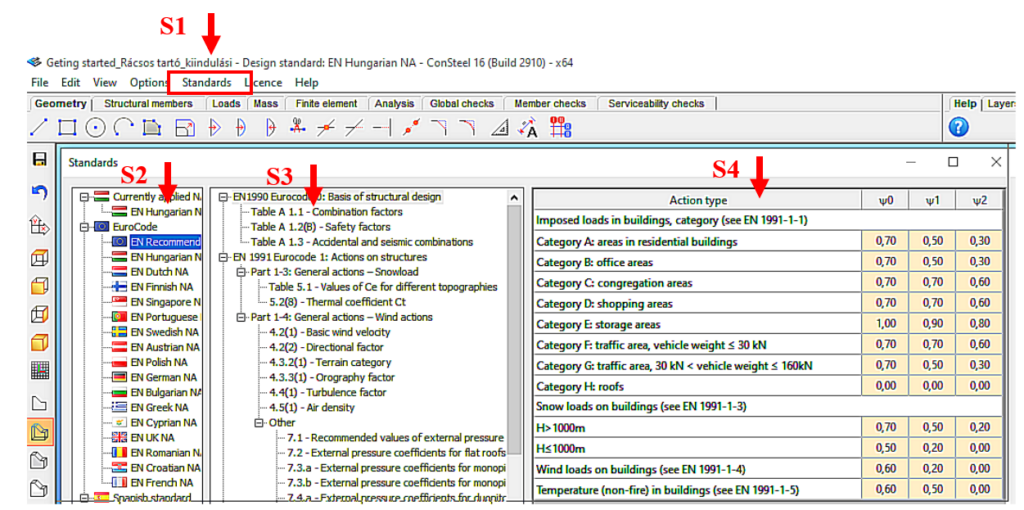
(S1: access standards; S2: select applicable standard; S3: select standard content; S4: display standard parameters).
The desired design standard can be selected from the list on the left of the panel. In this case, we select the EN Recommended option [S2]. The parameters applied by the selected standard can be accessed by selecting the corresponding row of the middle table [S3] of contents in the right-hand table [S4]. In Figure 2, the combination factors corresponding to Table 1.1 of the EC0 standard have been selected, whose parameters are shown in the right-hand table.
Setting the grid raster editor
First, let’s set the size of the raster according to the span of the structure by using the corresponding button [1] of the tool group on the left, which will bring up the Grid and Coordinate System adjustment panel (Figure 3).
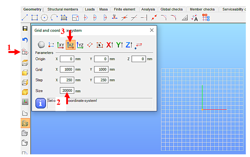
(1: set raster grid and coordinate system; 2: set raster occupancy size; 3: select view)
For example, for the 19.6m long support, the Size window can be set to 20000 millimeters [2]. To update the setting, press Enter. With the above setting, the raster will be 20m wide in X and Y directions, the raster line density will be 1000mm, and the step spacing will be 250mm. It is convenient to add the grid support model in the X-Z global coordinate plane, so the raster editor will be rotated to the X-Z plane. To do this, select the XZ plane option [3].
Loading initial cross-sections
One fundamental characteristic of general structural analysis programs is that they can only work with specifically defined cross-sections. Therefore, the first step is to choose the initial cross-sections for the task, according to the conceptual design. This may seem contradictory to the simple manual methods taught in basic statics courses, where the specific dimensions of the cross-section were often irrelevant information (e.g. calculation of internal forces). When using computer programs, however, we need to provide specific cross-sections even if their dimensions do not affect the static quantities to be calculated (e.g. in the present case, the normal forces of a truss beam). Nevertheless, we should aim to select cross-sections that match the geometrical size of the structure. In this case, the preliminary design served this purpose.
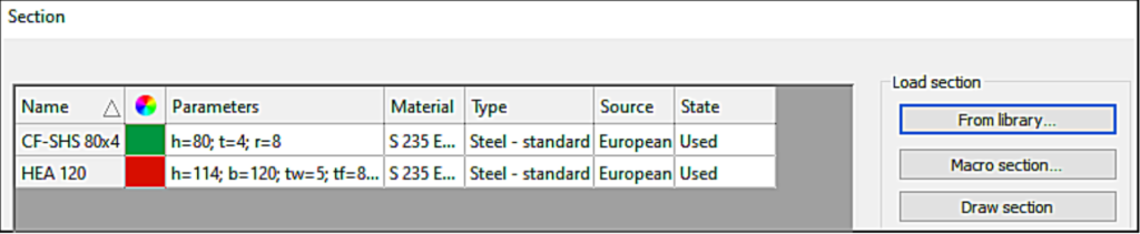
Initially, the section library for the current model is empty, so we first need to select the appropriate cross-sections. To do this, go to the Structure Members tab [4] and select the Section Administration option [5] on the left side of the horizontally positioned tool group, then select the “From Library…” button [6] in the panel that appears (Figure 4).
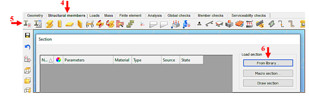
(4: picking up structural elements; 5: calling up the section control panel;
6: Select section type)
Figure 5 shows the loading of the HEA120 section, compliant with the European standard, which will be assigned to the chords. We select the region of the cross-section standard (European) and then its type (H profiles). From the list that appears, we can select the type of section (HEA) [7] and then the height of the section (120) [8]. By pressing the Load button [9], the program learns the cross-section, and from then on it knows everything about the cross-section and can work with it. Repeat the procedure as many times as you need different sections. Finally, the window is closed by pressing the Close button [10].
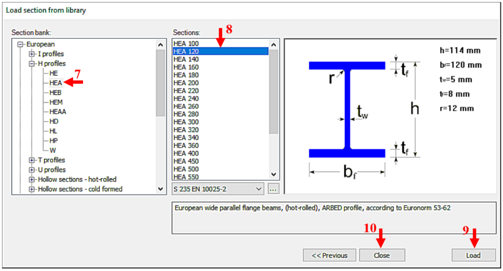
(7: select section type; 8: select section size; 9: scan selected section; 10: end loading process)
In our case, also a CF-SHS 80×4 closed section (from Library/Hollow sections – cold formed/CF-SHS/CF-SHS 80×4) was loaded for the bracing members (Figure 6).
Later on, you can obtain all the information about the cross-section using the Section module. To do this, select the cross-section in the table by clicking on the corresponding row and then click on Properties… to display all the properties of the cross-section, such as type data; cross-section characteristics, etc. The program works with two cross-section mechanical models in a dual manner. The GSS (General Solid Section) model [11] is used for static calculations and the EPS (Elastic Plate Segment) model [12] for standard design operations (Figure 7). The cross-sectional properties (surface area, moments of inertia, etc.) can be displayed by pressing the button [13].
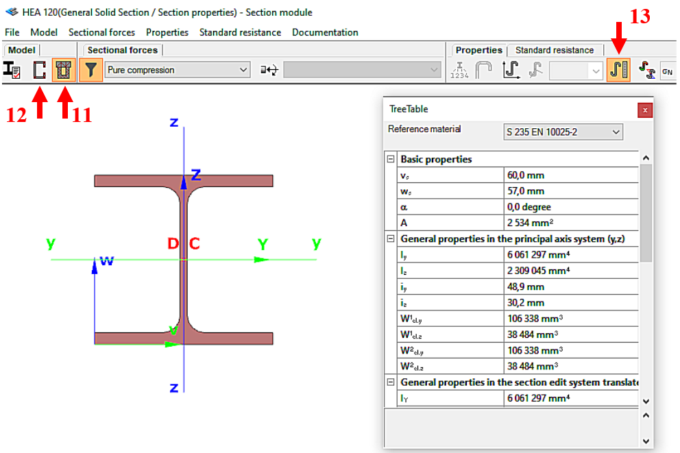
(11: Open GSS general section model; 12: Open EPS elastic plate segment model;
13: open cross-sectional properties table)
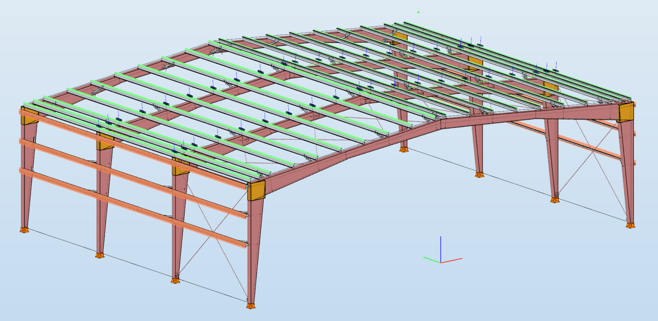
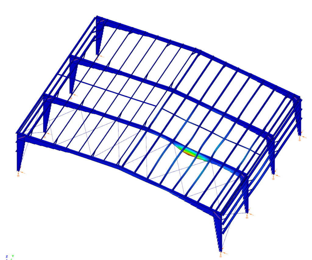
Did you know that you can use Consteel to design a pre-engineered Metal Building with all its unique characteristics, including web-tapered welded members, the interaction of primary and secondary structural elements, flange braces, shear and rotational stabilization effect provided by wall and roof sheeting?

Download the example model and try it!
Download modelIf you haven’t tried Consteel yet, request a trial for free!
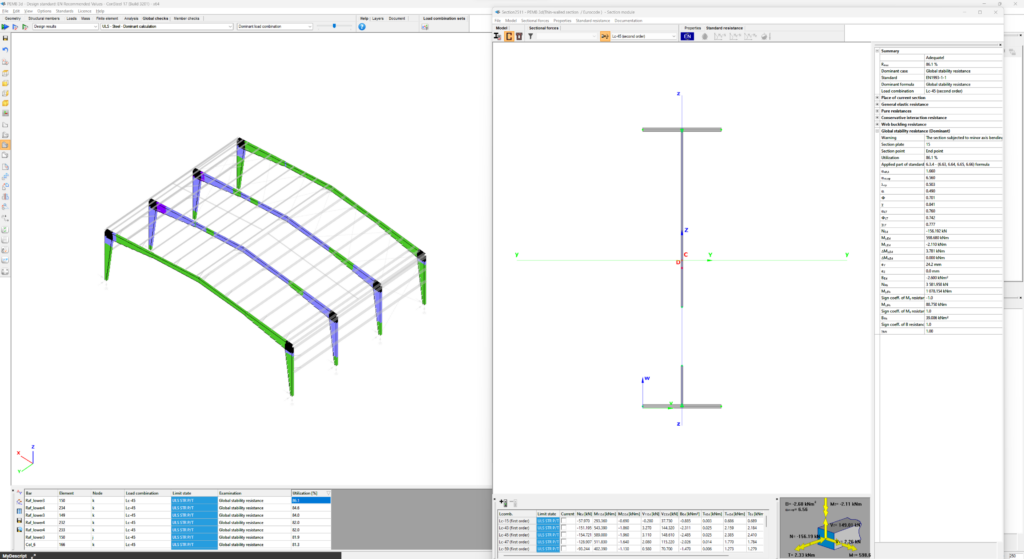
Try Consteel for freeThis overview delves into Consteel’s solution, offering an alternative approach to calculating effective cross-sectional properties and reshaping conventional methodologies in structural analysis and design.
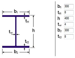
Determine the strength utilization of a double symmetric welded I cross-section with 384×4 web and 300×8 flanges, if the internal forces on the cross-section are NEd=500kN compressive force and My,Ed=100kNm bending moment. The material grade of the cross section is S235.
Calculation of cross-sectional properties
First, take the cross-section data (symmetric welded I-section), from which the Consteel software generates the EPS (and GSS) (see Online Manual/10.1.1 The EPS model) cross-section model (Fig. 1).
If the cross-section is class 4, the effective model is determined by the assumed normal stress distribution. According to EC3-1-1, the EPS model of a class 4 cross-section can be defined in two ways :
– method A: based on pure stress conditions,
– method B: based on complex stress condition.
In order to compare the results, the cross-section properties will be calculated by method A at first and then by method B.
Cross-sectional properties by method A
- pure compression NEd (Fig. 2):
Aeff=4720mm2
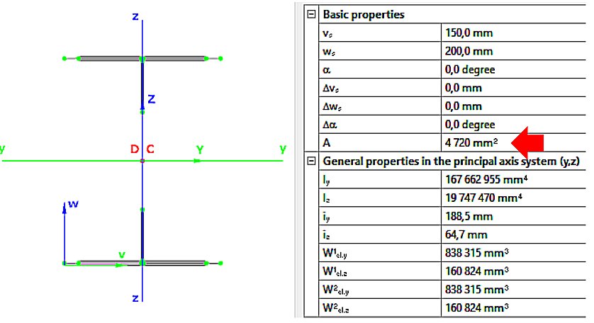
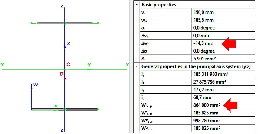
- pure bending My,Ed (Fig. 3):
Weff,y,min=864080mm3
ez=14.5mm
Cross-sectional properties by method B
GATEThe latest version, Consteel 17 is officially out! In 2023, our main focus for Consteel development is improving usability. New features prioritize efficient model manipulation, easy modification, and clear information presentation across Consteel, Descript, and our cloud-based platform, Steelspace. In this comprehensive video, we walk you through a step-by-step workflow guide, demonstrating how to leverage Consteel 17 to its full potential.
If you would like to delve deeper into the new features, check out our detailed blog post for an in-depth exploration of Consteel 17’s capabilities.