The evolution of compressed bar (column) design
One of the characteristic features of steel structures made of bars (e.g. lattice girders) is the compressed bar. We speak of a compressed bar when the structural element, which usually has a straight axis, is loaded by a compressive force P applied centrally (Figure 1).
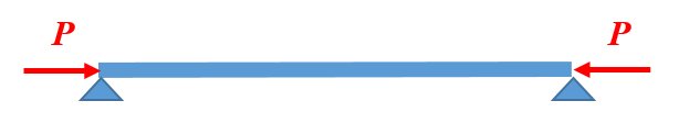
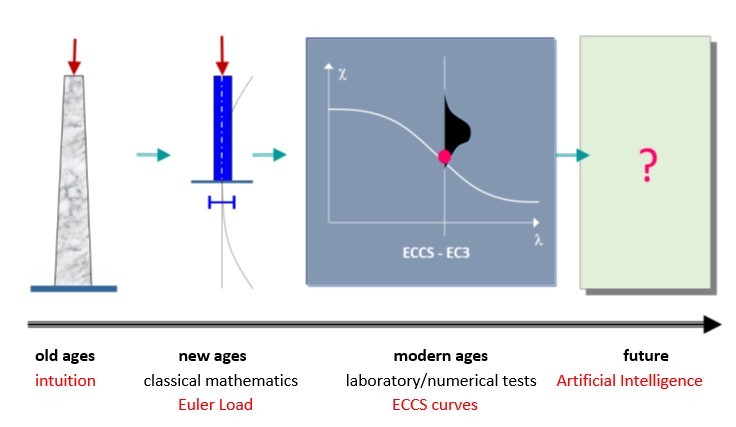
Figure 2 illustrates the evolution of compressed bar (column) design. In the beginning (in the old days), master builders determined the load-bearing capacity of compressed columns of different materials and sizes on the basis of the experience accumulated over the centuries, passed down from master to apprentice. A significant change was brought about by the application of classical mathematical differential analysis to engineering. The Swiss mathematician and physicist Euler (1707-1783) solved the problem of the deflection of a compressed elastic line, which could be applied to the solution of the elastic compressed bar (Euler’s force). In the following centuries, engineers recognised that Euler’s force only gave an acceptable approximation to the real load capacity of a compressed bar in certain cases (mainly for large slender bars). Many solutions for the bearing capacity of a compressed bar were developed that were more advanced than the Euler formula, but it was not until the huge structural engineering boom following World War II that significant changes were made. Compression bar experiments were carried out in every major structural laboratory in the world, and a database of over two thousand experiments was compiled from the results. The load capacity of the pressure bar was given by a formula based on the database, using the method of mathematical statistics.
This methodology is still dominant today: ‘the dimensioning of the compressed bar has become a political issue for the steel construction profession…’. Understanding the principle of compressed bar design is therefore essential for the structural engineer.
The right side of the Figure 2 also contains a hint for the future. At the level of scientific research, it is already present that the load capacity of a real compressed column can be determined by mathematical-mechanical simulation. Indeed, in the near future, databases that go beyond anything we know today can be created using supercomputers. On the basis of such a gigantic database, artificial intelligence could, at least in principle, supersede existing engineering knowledge and methodology. But the reality is that structural engineering is not one of the pull sectors (such as the defense or automotive industries), so this new shift in design theory is certainly a long way off.
In the following, the Euler force and the experimentally based standard design formula, which are of major importance to structural steel engineering today, are discussed in detail.
Buckling strength of the ideal columns: the Euler force
Assume that the hinged compressed column shown in the Figure 3 has the following properties:
- perfectly straight,
- its material is perfectly linearly elastic,
- centrally compressed.
Under the above conditions, perform the compressed column experiment using Consteel software: run the Linear Buckling Analysis (LBA) calculation. The result is illustrated in Figure 3.
gateTheoretical background
According to the beam-column theory, two types of torsional effects exist.
Saint-Venant torsional component
Some closed thin-walled cross-sections produce only uniform St. Venant torsion if subjected to torsion. For these, only shear stress τt occurs.
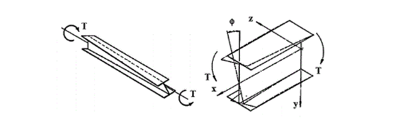
The non-uniform torsional component
Open cross-sections might produce also normal stresses as a result of torsion.[1.]
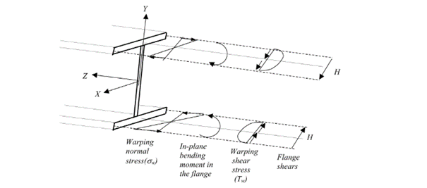
Warping causes in-plane bending moments in the flanges. From the bending moment arise both shear and normal stresses as it can be seen in Fig. 2 above.
Discrete warping restraint
The load-bearing capacity of a thin-walled open section against lateral-torsional buckling can be increased by improving the section’s warping stiffness. This can be done by adding additional stiffeners to the section at the right locations, which will reduce the relative rotation between the flanges due to the torsional stiffness of this stiffener. In Consteel, such stiffener can be added to a Superbeam using the special Stiffener tool. Consteel will automatically create a warping support in the position of the stiffener, the stiffness of which is calculated using the formulas below. Of course, warping support can also be defined manually by specifying the correct stiffness value, calculated with the same formulas (see literature [3]).
The following types of stiffeners can be used:
- Web stiffeners
- T – stiffener
- L – stiffener
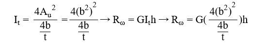
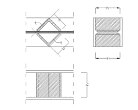
- Box stiffener
- Channel –stiffener
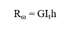
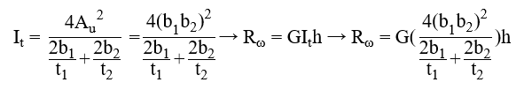
The general formula which can be used to determine the stiffness of the discrete warping restraint is the following:
where,
Rω = the stiffness of the discrete warping restraint
G = shear modulus
GIt = the Saint-Venan torsional constant
h = height of the stiffener
Effect of the different stiffener types
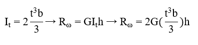
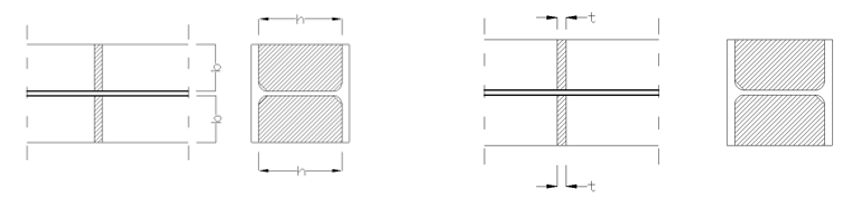
Web stiffener
where
b = width of the web stiffener [mm]
t = thickness of the web stiffener [mm]
h = height of the web stiffener [mm]
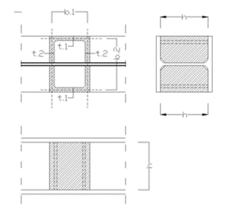
T – stiffener
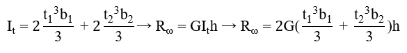
where
b1 = width of the battens [mm]
t1 = thickness of the battens [mm]
b2 = width of the web stiffener [mm]
t2 = thickness of the web stiffener [mm]
h = height of the web stiffener [mm]
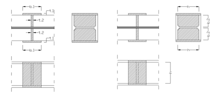
L-stiffener
where
b = width of the L-section [mm]
t = thickness of the L-section [mm]
h = height of the L-section [mm]
Channel stiffener
where
b1 = width of channel web [mm]
t1 = thickness of channel web [mm]
b2 = width of channel flange [mm]
t2 = thickness of channel flange [mm]
h = height of the web stiffener [mm]
Numerical example
The following example will show the increase of the lateral-torsional buckling resistance of a simple supported structural beam strengthened with a box stiffeners. The effect of such additional plates can be clearly visible when shell finite elements are used.
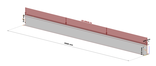
Shell model
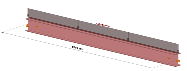
Fig. 7 shows a simple fork supported structural member with welded cross-section modeled with shell finite elements and subjected to a uniform load along the member length acting at the level of the top flange.
Table 1. and Table 2. contain the geometric parameters and material properties of the double symmetric I section. The total length of the beam member is 5000 mm, the eccentricity of the line load is 150 mm in direction z.
| Name | Dimension | Value |
|---|---|---|
| Width of the top Flange | [mm] | 200 |
| Thickness of the top Flange | [mm] | 10 |
| Web height | [mm] | 300 |
| Web thickness | [mm] | 10 |
| Width of the bottom Flange | [mm] | 200 |
| Thickness of the bottom Flange | [mm] | 10 |
Table 1: geometric parameters
| Name | Dimension | Value |
|---|---|---|
| Elastic modulus | [N/mm2] | 200 |
| Poisson ratio | [-] | 10 |
| Yield strength | [N/mm2] | 300 |
Table 2: material properties
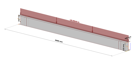
Box stiffener
The box stiffeners are located near the supports as can be seen in Fig. 8. Table 3. contains the geometric parameters of the box stiffeners.
| Name | Dimension | Value |
|---|---|---|
| Width of the web stiffener | [mm] | 100 |
| Thickness of the battens | [mm] | 100 |
| Total width of the box stiffener | [mm] | 200 |
| Height of the plates | [mm] | 300 |
| Thickness of the plates | [mm] | 10 |
Table 3: geometric parameters of the box stiffeners
7DOF beam model
The same effect in a model using 7DOF beam finite elements can be obtained when discrete warping spring supports are defined at the location of the box stiffeners.
Discrete warping stiffness calculated by hand
gateThis article aims to cover the theoretical background of the shear field stiffness determination methods implemented in Consteel. Modeling with the shear field stiffness based method will also be compared with shell modeling of trapezoidal deckings in Consteel.
Theoretical background
Modeling the shear stiffness of trapezoidal deckings is used to utilize their contribution to stabilizing the main structure. The possibility to consider the shear stiffness of sheetings is implemented at finite element level in Consteel and ensures easy modeling through its application onto beam elements.
Shear panel definitions
For the discussion let’s establish some basic definitions regarding shear panels.
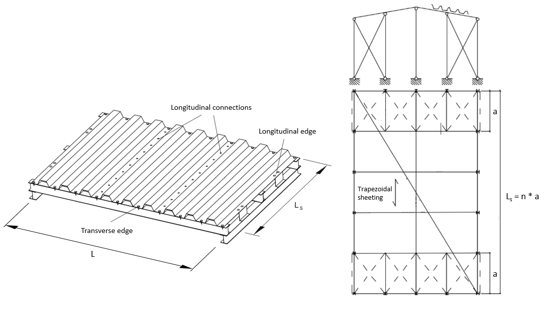
- Dimensions:
- L [m]: width of the shear field, also the span of the stabilized beam
- Ls [m]: complete length of the shear field parallel to the ribs
- a [m]: effective shear field length for only one connecting beam element
- Stiffnesses:
- Gs [kN/m]: specific shear stiffness considering a 1 m long strip of an “Ls“ long shear field
- S [kN]: shear stiffness of the complete shear field
Determaination of the shear field stiffness
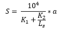
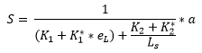
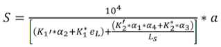
The general formula to calculate the shear stiffness in Consteel is the following:

There are 4 methods implemented in Consteel to determine the shear field stiffness:
- Schardt/Strehl method: (K1, K2), DIN 18807-1:1987-06 [1]
- improved Schardt/Strehl method: (K1, K2, K1*, K2* and eL)
- Bryan/Davies method: (K1, K2, K1*, K2*, eL, α1, α2, α3, α4)
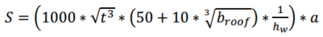
- Eurocode 3: (1993-1-3 10.1.1 (10)) [2]
See in more detail here: Determination of shear field stiffness and application in Consteel
The first 3 methods are based on the 1. one, the Schardt/Strehl method. These methods operate on the same principle by calculating the shear stiffness from values (K1, K2, etc.) provided by the manufacturer of the sheetings. The 2. and 3. methods are more developed versions of the 1. one, trying to more accurately calculate the shear stiffness by introducing additional parameters to account for more sources of the overall shear stiffness of the sheeting.
The 4. method that is found in Eurocode 3 can be more generally applied since that doesn’t require such product specific values.
A basic assumption in case of these methods is that the sheeting is connected at every rib to the beams that it stabilizes (purlins in most cases). An additional modifying factor in case of all these methods is if the trapezoidal sheeting is not fixed at every rib, but every second rib, then the final “S” shear stiffness should be substituted by 0,2*S.
Theoretical background of the Schardt/Strehl method
This approach is based on a model assuming a fully linear elastic behaviour of the diaphragm. The ultimate limit state is therefore defined by yielding in the corner radius at the flange-web transition. The mechanical model also assumes that the sheeting is fixed to the substructure at all 4 edges. Shear forces RQ and RL are acting on the sheeting at the individual fixed points on the lower flanges where the sheeting is screwed to the substructure. The number of waves in the sheeting is assumed to be large enough so that the individual forces acting at the transverse edges in the middle are assumed to be constant (n>10). The length “Ls” of the shear field can be arbitrary, but should be in reasonable proportion to the width “L” of the shear field (<4).
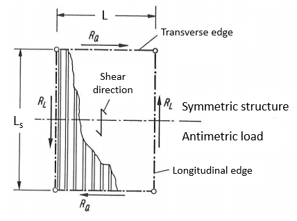
Based on these assumptions the mechanical analysis can be isolated to a half of one wave of the sheeting as shown on the left-hand side of the following figure:
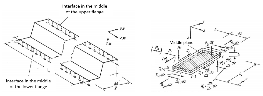
On the right-hand side the considered internal forces are shown for one slice of the sheeting.
Assumptions for the mechanical model:
- The Ms and Mz moments are neglected (shown in brackets on the right-hand side figure).
- Transverse bending moments “mi” at the level of the plate are considered. These moments have a 0 value in the center of the lower and upper flanges.
- The longitudinal stresses σz are constant over the thickness “ti” of the plates and linearly distributed over the height “hi”.
- The flexibility of connections is neglected.
The method accounts for the following effects:
- Shear deformation: corresponding value: K1 [m/kN] shows the sheetings compliance coming from shear deformation. The lower this value is, the more stiffness the sheeting has.
- Warping deformation: corresponding value: K2 [m2/kN] shows the sheetings compliance coming from warping deformation. The lower this value is, the more stiffness the sheeting has.
Component considering shear deformation
The value K1 can be calculated from the following formula based on the properties of the trapezoidal sheeting:
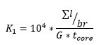
where
- ∑l [mm]: Summed up length of all the plates within one full wave
- br [mm]: length of one complete wave
- G [N/mm2]: shear modulus
- tcore [mm]: structural thickness. (generally: tcore = tnominal – 0,04 mm)
The formula of the K1 value is similar to how it should be calculated in case of a planar plate, but its thickness corrected with the ∑l/br ratio, or in other words the ratio of the complete length of the plates to the length of one wave. The K1 shear deformation compliance value is directly proportional to the ∑l/br ratio, therefore if a certain trapezoidal sheetings height is increased with everything else left the same, the corresponding K1 value would increase, and the stiffness coming from shear deformation would decrease. On the other hand the K1 value is inversely proportional to “G” shear modulus and “tcore“ structural thickness, so if either of these values would increase, K1 would decrease, and the stiffness coming from shear deformation would increase.
Component considering warping deformation
The K2 parameter further softens the structure taking into account the warping deformations. The detailed calculation of the K2 parameter will not be shown here due to its extensiveness and complexity. The details of this calculation can be found in the literature [5]. The calculation is based on the “Folded Plate” theory [8]. To obtain the K2 parameter the warping displacements and warping coordinates have to be calculated for the sheeting. The following figure shows an example for the normalized warping displacements and deformed shapes for k=1 and k=2:
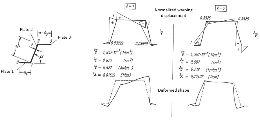
k=1 and k=2 are connected to individual solutions for the differential equation system describing the mechanical behavior based on the “Folded Plate” theory.
Calculating shear stiffness
The behavior of the two components in the formula of the shear stiffness is different. The part that considers the shear deformation only depends on the effective width “a”, but independent from the total length of the shear field “Ls”. On the other hand the part that considers the warping deformation is also dependent on the total length of the shear field “Ls”. The K2 parameter in the denominator is divided by Ls, which means that the longer the total shear field is, the larger the specific shear stiffness is going to get because of the contribution of the warping deformations.
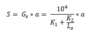
Also if the total length of the shear field “Ls“ would get really low, then K2/Ls would approach infinity, which means that the stiffness approaches zero. For this reason a minimal length for sheetings “Ls,min” is also provided by the manufacturers, which gives the specific shear stiffness “Gs” a minimum value.
Comparison against shell models
The effect of the shear stiffness of a trapezoidal sheeting can be modeled in multiple ways. In Consteel additionally to built-in shear field field object applicable on beam elements, the sheeting can be modeled directly with shell elements. This latter approach is more complicated and time consuming to set up, but should provide similar results. Such a comparison was prepared in Consteel.
Examined structure
Stabilized beam: IPE300 S235
Span: L = 4140 mm
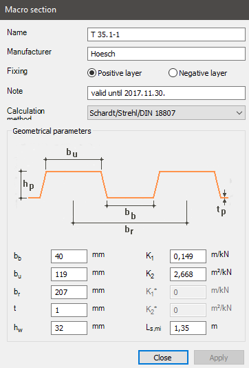
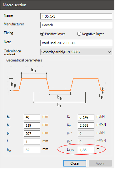
Type of trapezoidal sheeting: Hoesch T 35.1
- Examined thicknesses: 0,75 mm; 1 mm; 1,25 mm
- Examined sheeting lengths: 2 m, 3 m
Horizontal line load: qy = 10 kN/m
The load and the trapezoidal sheeting are both acting on the centerline of the stabilized beam.
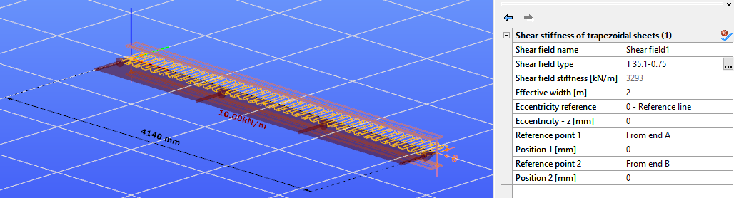
Consteel shear field model
In this modeling version the stabilizing effect of the trapezoidal sheeting is modeled by the shear field object implemented into Consteel.
Example figure: Ls = 2 m, a = 2 m, Gs = 3293 kN/m, S = 6586 kN
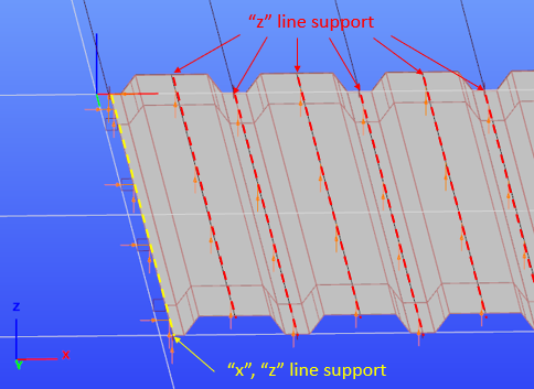
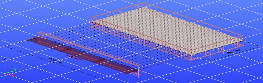
Consteel shell model
In this modeling version, the trapezoidal sheeting is modeled by shell elements. The thicknesses of the shell elements are equal to the structural thickness tcore. The model of the trapezoidal sheeting is included in a frame made from beam elements. The sheeting is connected to the frame by link elements at the lower flanges where the sheeting is screwed to the substructure. The frame is included in the model in order to connect the shell elements to the main beam. The beams of the frame have a cross-section that has relatively insignificant weaker axis inertia compared to the shear stiffness of the sheeting. The shell elements are connected through the frame to the main beam by link elements that only transfer force in their axial direction.
Example figure: Ls = 2 m, a = 2 m
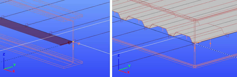
The shell elements are also supported in the vertical direction along the middle lines of its top and bottom flanges in order to eliminate the bending deformation resulting from the eccentric compression load on the sheeting, since the shear field model also does not take this effect into account. The edges on both sides of the sheeting are supported against “x” and “z” directional displacements in order to account for the sheeting being fixed to the substructure at all 4 of its edges. The line supports on the plate elements are shown on the following picture viewing the structure from below.