Introduction
This article presents the calculation method for determining the buckling resistance of a pinned column with intermediate restraints in accordance with Eurocode standards. The procedure is based on an example from the Access Steel design examples collection and is compared with the calculation process implemented in Consteel’s steel member design functions, specifically within the Member Checks module.
In the following sections, a step-by-step guide is provided to demonstrate how the member check functionality can be applied to simple cases, highlighting both methodology and practical usage.
Input Data for the Example
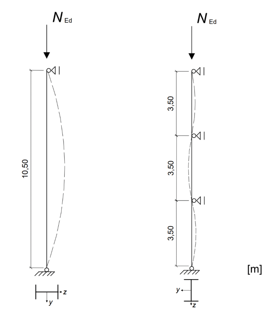
The example considers a pinned column in a multi-storey building, subjected to a design axial force of $N_{Ed}$ = 1000 kN. The column has a total length of 10.50 m and is laterally restrained about the y–y axis at intervals of 3.50 m.
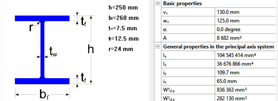
The member is a rolled HEA 260 section made of S235 steel. The cross-section is classified as Class 1. The geometric properties of the section are: height h = 250 mm, width b = 260 mm, web thickness $t_w$ = 7.5 mm, flange thickness $t_f$ = 12.5 mm, and fillet radius r = 24 mm. The cross-sectional area is A = 86.8 cm², with moments of inertia $I_y$ = 10450 cm⁴ and $I_z$ = 3668 cm⁴.
The material properties are defined according to EN 1993-1-1. Since the maximum thickness is less than 40 mm, the yield strength is taken as $I_y$ = 235 N/mm². The partial safety factors are γM0 = 1.0 and γM1 = 1.0.
Determining Design Buckling Resistance of a Compression Member
The design buckling resistance of the column $N_{b,Rd}$ is evaluated by determining the reduction factor χ for both principal buckling directions. This requires the calculation of the elastic critical forces $N_{cr}$, which form the basis for identifying the governing buckling mode.
Elastic critical force for the relevant buckling mode $N_{cr}$
The Young’s modulus is taken as $E=210000 \frac{N}{mm^2}$. The buckling lengths in the respective planes are $L_{cr,y} = 10.50m$ for buckling about the y–y axis and $L_{cr,z} = 3.50m$ for buckling about the z–z axis. Observe that the buckling lengths for the strong and weak axes differ according to the support conditions, which must be determined by the engineer in manual calculations.
$$N_{cr,y}=\frac{π^2*E*I_{y}}{L_{cr,y^2}}=1964.5 kN$$
$$N_{cr,z}=\frac{π^2*E*I_{z}}{L_{cr,z^2}}=6206.0 kN$$
In Consteel, the elastic critical force for the relevant buckling mode can be determined using the Individual Member Design approach. This is accessible in the Member Checks tab under the Steel module, where selected members can be added and evaluated.

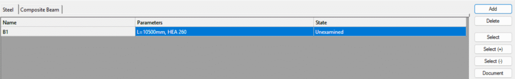
Once a member is selected, the analysis results are automatically loaded, provided that first- or second-order analysis results are available. Ensure that the analysis has been run in the Analysis tab and the cross section check on the Global ckecks tab before proceeding to the Member Checks section.
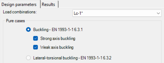
For the pinned column with intermediate restraints, the relevant buckling cases, strong and weak axis, are selected, and the dominant load combination is automatically indicated with a *. Consteel identifies the intermediate restraints separately for each direction and divides the member into segments accordingly to help determine the correct buckling lengths.
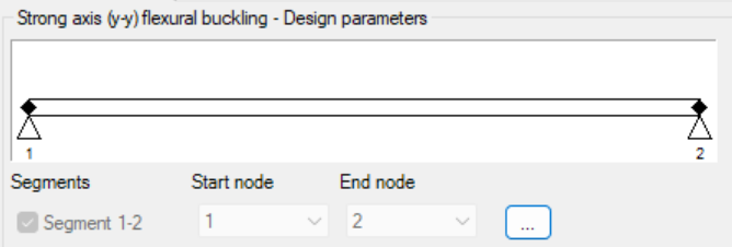
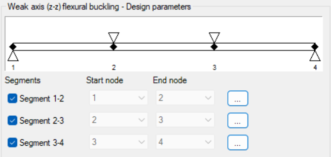
Design parameters for each segment are set with the three-dot icon:
At this step, users must verify the assigned values. By default, the first value is applied, and the correct buckling shape or effective length factor should be confirmed based on engineering judgment.
In order to use the critical load multiplier selection option, make sure to perform the calculation first:


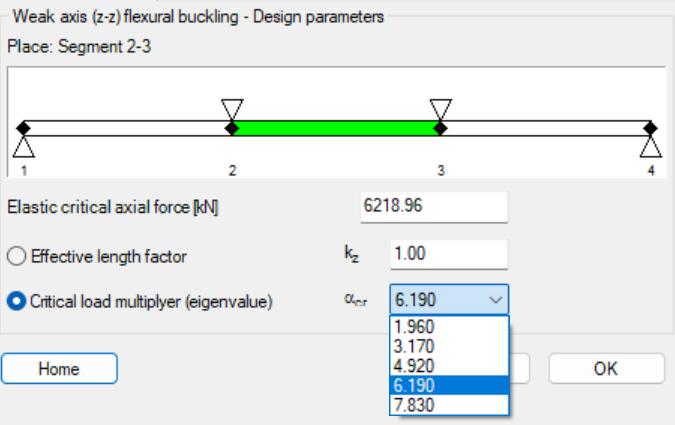
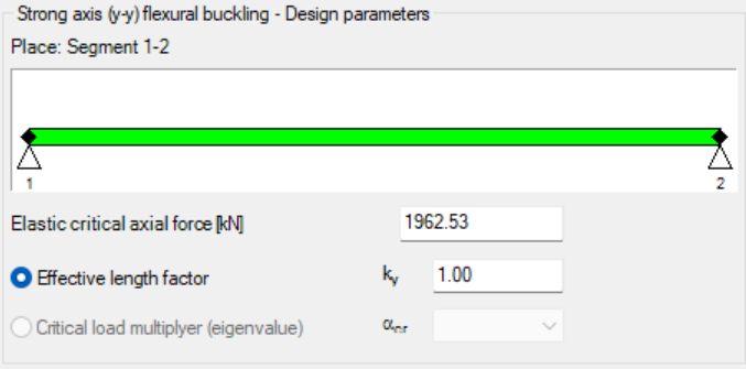
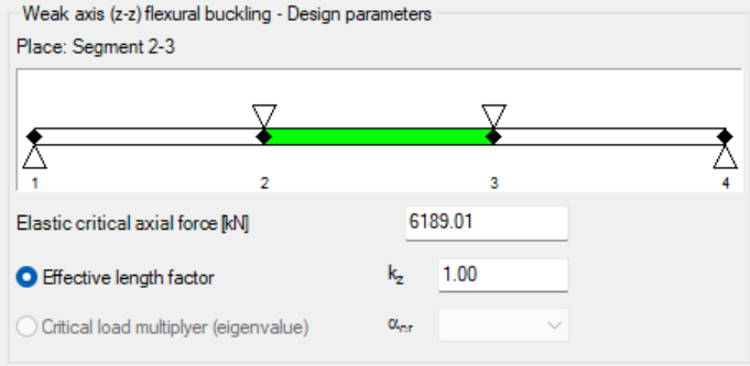
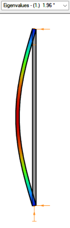
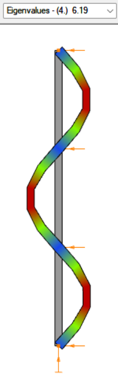
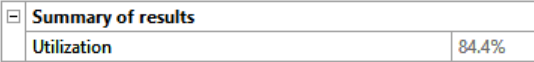
In order to check whether the correct critical load multiplier was selected, you can examine the effective length factor, which is calculated based on it (in this case, it is 1 for both directions). In our example, the relevant buckling shapes for the y–y and z–z directions are as follows:
The elastic critical force $N_{cr}$ is calculated automatically, regardless of whether the effective length factor was entered manually or the critical load multiplier was selected.
| Access Steel – manual calculation | Consteel using the effective length factor | Consteel using the critical load multiplier | |
| $N_{cr,y}$ | 1964.5 kN | 1962.53 kN | 1973.76 kN |
| $N_{cr,z}$ | 6206.0 kN | 6189.01 kN | 6218.96 kN |
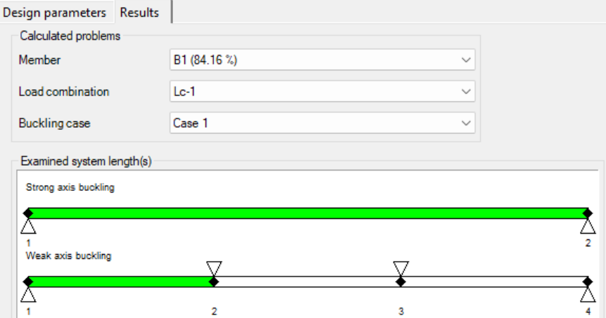
Once all parameters are defined, the design check is executed by clicking the Check button, and the results are displayed.
Results can be reviewed and filtered by member, load combination, and buckling case. Lateral-torsional buckling checks follow a similar procedure, with segment boundaries adjustable and critical moments calculated either analytically or using the critical load multiplier.
Non-dimensional slenderness
In order to determine the reduction factor, the non-dimensional slenderness λ must be calculated based on the elastic critical force corresponding to the relevant buckling mode.
$$\overline{\lambda_y} = \sqrt{\frac{A*f_y}{N_{cr,y}}}=\sqrt{\frac{86.8*23.5}{1965}}=1.016$$
$$\overline{\lambda_z} = \sqrt{\frac{A*f_z}{N_{cr,z}}}=\sqrt{\frac{86.8*23.5}{6206}}=0.573$$
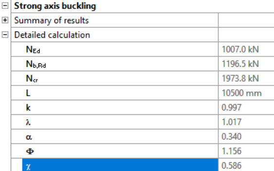
In Consteel, the detailed calculations for strong and weak axis buckling can be reviewed separately on the Results tab:
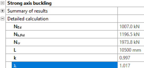
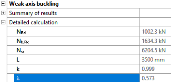
Reduction factor
For axial compression, the value of χ corresponding to the relevant non-dimensional slenderness $\overline{\lambda}$ should be determined from the appropriate buckling curve in accordance with EN 1993-1-1 §6.3.1.2.
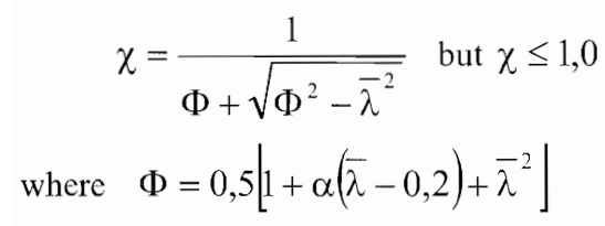
For $\frac{h}{b}= \frac{250mm}{260mm} = 0.96 < 1.2$ and $t_f = 12.5 mm< 100 mm$
- buckling about axis y-y, buckling curve b, imperfection factor $\alpha=0.34$
$$\varphi_y=0.5*[1+0.34(1.019-0.2)+1.019^2]=1.158$$
$$\chi_y=\frac{1}{1.158+\sqrt{1.158^2-1.019^2}}=0.585$$
- buckling about axis z-z, buckling curve c, imperfection factor $\alpha=0.49$
$$\varphi_y=0.5*[1+0.49(0.573-0.2)+0.573^2]=0.756$$
$$\chi_y=\frac{1}{0.756+\sqrt{0.756^2-0.573^2}}=0.801$$
$$\chi=min(\chi_y;\chi_z)$$
$$\chi=0.585<1.00$$
Design buckling resistance of a compression member
$$N_{b,Rd}=\chi*\frac{A*f_y}{\gamma_{M1}}=0.585*\frac{86.8*23.5}{1.0}=1193 kN$$
$$\frac{N_Ed}{N_{b,Rd}}=\frac{1000}{1193}=0.84<1.00$$
Conclusion
This example demonstrates the application of the isolated member approach for a simple compression member. For more complex cases or alternative stability verification methods, such as the imperfection approach or the general method, refer to the dedicated article on stability design methods, where their principles and applications are discussed in detail.
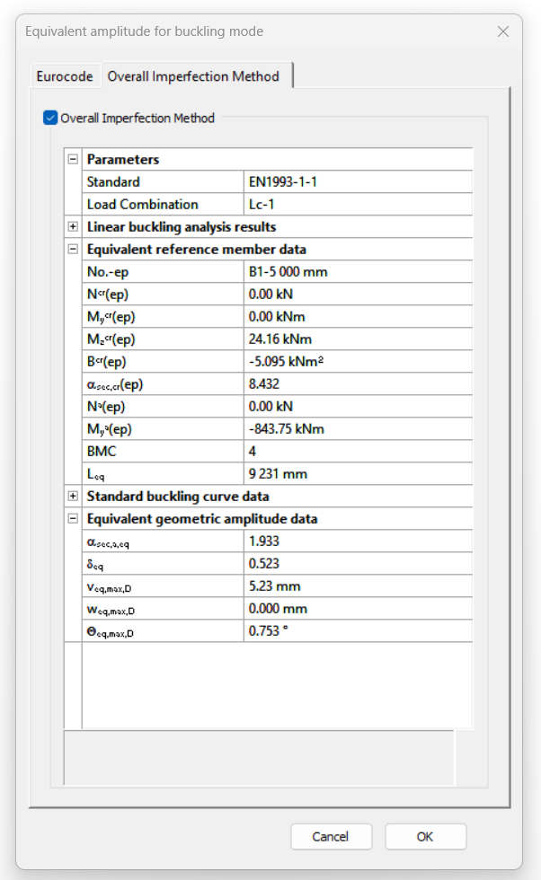
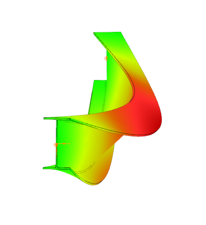
Download modelConsteel recommends to use the General Method from EN 1993-1-1 for the evaluation of out-of-plane strength of members and sturctures. In addition, the scaled imperfection based 2nd order approach is available.
Did you know, that when linear buckling eigenform affine imperfections are used, Consteel can scale automatically the selected eigenmodes to perform a Eurocode compatible design? And you can even combine several imperfections?
Download the example model and try it!
Bending:
Download modelCopmression:
Download modelIf you haven’t tried Consteel yet, request a trial for free!
Try Consteel for free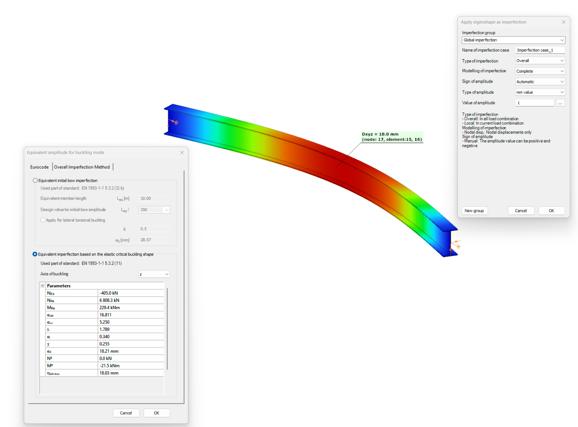
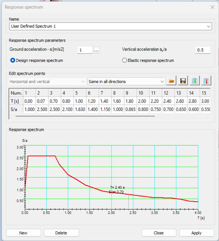
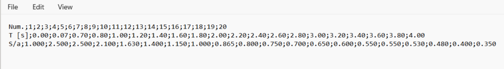
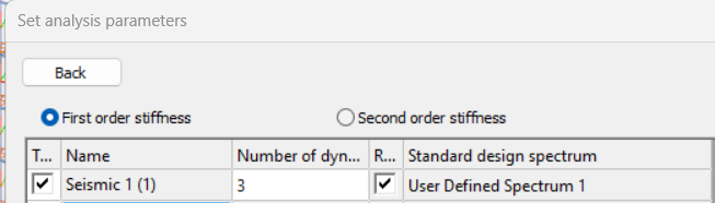
Did you know that in addition the standard Type 1 and Type 2 response spectrums defined by Eurocode 8, you can use also user-defined spectrums with Consteel?
Download the example model and try it!
Download modelIf you haven’t tried Consteel yet, request a trial for free!
Try Consteel for free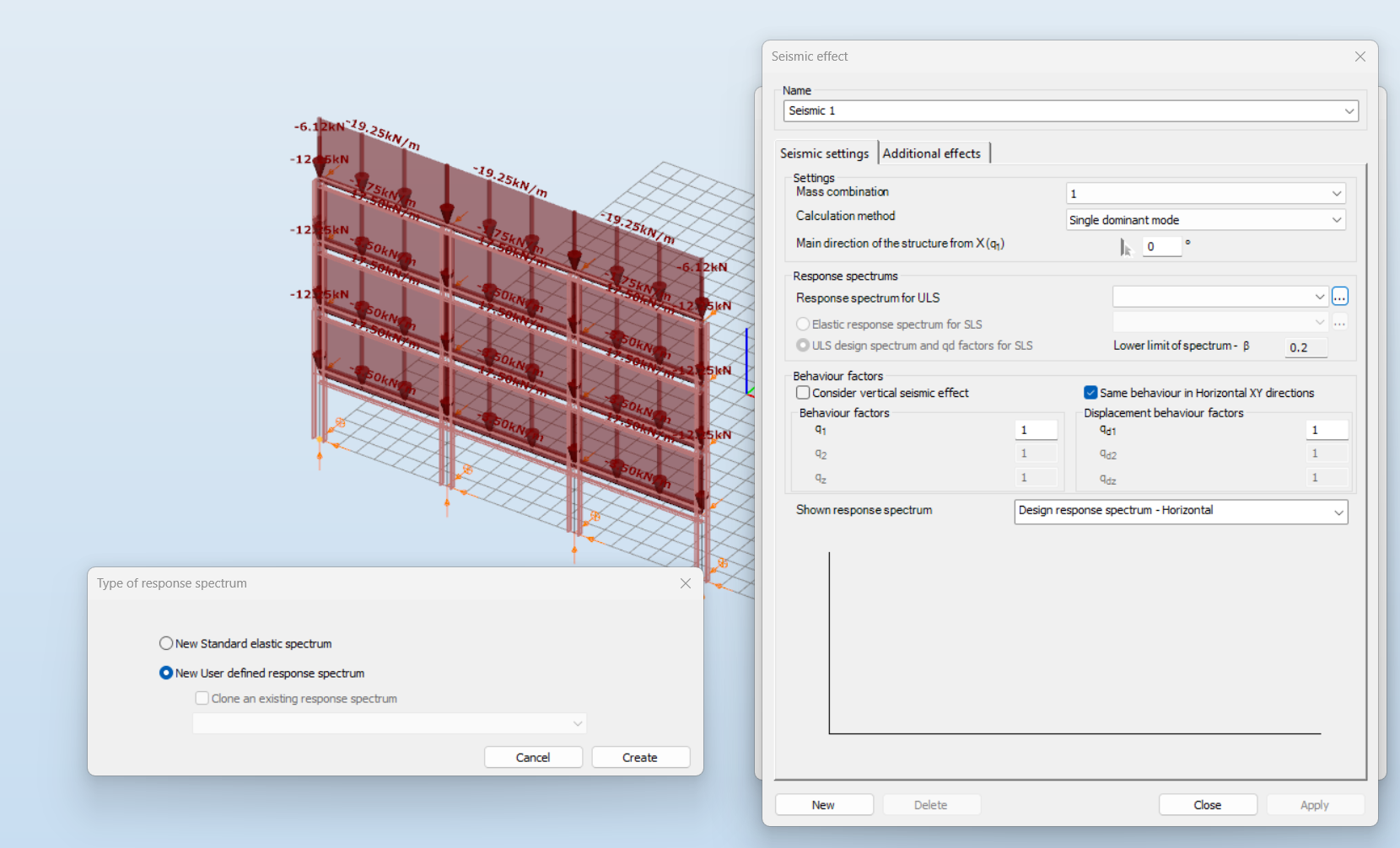

Bevezetés
Amennyiben a síkban hajlított gerenda szabadon elmozdulhat és elcsavarodhat a két támaszpontja között, akkor a lehajlás mellett hirtelen merőleges elmozdulás és elcsavarodás jöhet létre: a gerenda kifordul a síkjából. Ezt a jelenséget szemlélteti az 1. ábra, amely egy kéttámaszú, az erős tengely körül hajlított I keresztmetszetű gerendát mutat: a függőleges síkban történő hajlítás során, amikor a nyomaték elér egy kritikus értéket, a gerenda hirtelen oldalirányban elmozdul és elfordul a két támasz között. Ez a jelenség a kifordulás, amely stabilitásvesztési mód a tökéletes gerendára és a valódi gerendára egyaránt vonatkozhat.
A gerenda kifordulással szembeni méretezése teljes mértékben analóg a nyomott oszlop kihajlási elleni méretezésével. Az analógiát az 1. táblázat szemlélteti, ahol feltüntettük a kihajlási és a kifordulási ellenállást befolyásoló, egymásnak megfelelő paramétereket.
| Kihajlás | Kifordulás |
|---|---|
| tervezési nyomóerő ($N_{Ed}$) | tervezési nyomaték ($M_{Ed}$) |
| kritikus erő ($N_{cr}$) | kritikus nyomaték ($M_{cr}$) |
| kihajlási karcsúság ($\frac{}{\lambda}$) | kifordulási karcsúság ($\frac{}{\lambda}_{LT}$) |
| kihajlási csökkentő tényező ($\chi$) | kifordulási csökkentő tényező ($\chi_{LT}$) |
| kihajlási ellenállás ($N_{b,Rd}$) | kifordulási ellenállás ($M_{b,Rd}$) |
A tökéletes gerenda kritikus nyomatékát a My,Edtervezési hajlítónyomaték-diagram maximális értékének helyén kell meghatározni. Kétszeresen szimmetrikus I keresztmetszet esetén:
$$M_{cr}=C_1\frac{\pi^2EI_z}{(k_z⋅L)^2}\left[\frac{I_\omega }{I_z}+ \frac{(k_zL)^2GI_t}{\pi^2EI_z}\right] ^{0.5} $$
ahol kz a keresztmetszet gyenge tengelye körüli befogási tényező, G a nyírási modulus, It és Iω pedig a keresztmetszet tiszta (St. Venant) és gátolt csavarási tehetetlenségi nyomatéka. A C1 tényező értéke a hajlító nyomatéki diagram alakjától függ, az értéke megfelelő táblázatokban és kézikönyvekben megtalálható. Konstans nyomatéki ábra esetén C1=1.0. A többi tervezési paraméter, különösen a $\chi_{LT}$ kifordulási csökkentő tényező képlete a figyelembe vett tervezési szabványtól függ.
Kifordulási ellenállás az EN1993-1-1 szerint
A hajlított gerenda kifordulás elleni méretezését (teherbírás-ellenőrzést) az EC3-1-1 szerint a következő lépésekben kell elvégezni:
gateRácsos tartó szerkezet méretezése
A rácsos tartók globális (rúdszerkezeti szintű) méretezése nem igényel különleges elméleti ismeretet: rendszerint a hajlítónyomatékok és a nyíróerők elhanyagolásával a rácsos tartók rudjait nyomott és/vagy húzott rúdként méretezzük. A nyomott rudak méretezését manapság modell alapú számítógépes eljárással hajtjuk végre. Ennek részleteit lásd a Nyomott rúd méretezése kihajlás ellen című tudásbázis anyagban. Itt csak a nyomott rudak kihajlási hosszának meghatározását mutatjuk be.
A nyomott rúd méretezésénél a legfontosabb paraméter a rúdkarcsúság:
$$\overline{\lambda}=\sqrt\frac{Af_y}{N_{cr}}$$
ahol
$$N_{cr}=\frac{\pi^2El}{(kL)^2}$$
ahol a k kihajlási hosszt (befogási tényezőt) az EN1993-1-1 szabvány, a kézi számítások megkönnyítése érdekében, az alábbiak szerint javasolja felvenni:
| Nyomott rúd típusa | Kihajlás iránya | k |
|---|---|---|
| övrúd | – tartó síkjában – tartó síkjára merőlegesen | 0.9 0.9 |
| rácsrúd | – tartó síkjában – tartó síkjára merőlegesen | 0.9 1.0 |
A modell alapú számítógépes eljárásokon alapuló szoftverek (pl. a Consteel szoftver) a fenti konzervatív szabály helyett az Ncr rugalmas kritikus erőt közvetlenül végeselemes numerikus módszerrel, a teljes rácsos tartó viselkedésének figyelembe vételével, határozzák meg. Az alábbi példával a szabvány által javasolt kézi méretezési eljárás és a modern, modell alapú numerikus eljárás eredményének viszonyát kívánjuk szemléltetni.
- Legyen a vizsgált rácsos tartó szerkezeti modellje az 1. ábrán látható Consteel modell.
- A feltűntetett teher feleljen meg a tartó mértékadó tervezési teherkombinációjának.
- Határozzuk meg a legjobban igénybe vett nyomott övrúd kihajlási hosszát végeselemes numerikus stabilitási analízis segítségével.
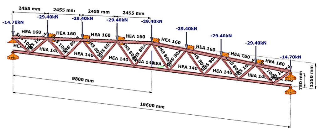
(Consteel szoftver)
Eljárások összehasonlítása
A számítás lépései a következők:
Rugalmas stabilitási analízis
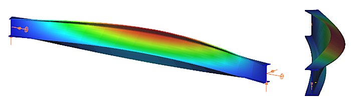
A rugalmas modell stabilitási analízise megmutatja, hogy a rácsos szerkezet mértékadó stabilitásvesztési módját és az ahhoz tartozó αcr rugalmas kritikus teherszorzót (2. ábra).
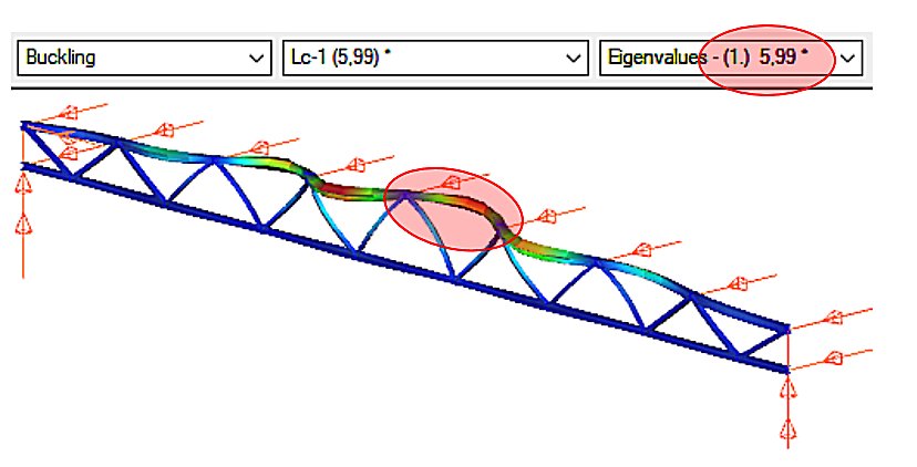
Láthatjuk, hogy a terhelés hatására a tökéletesen rugalmas modell felső öve oldalsó irányban kihajlást szenved. A teher, amely hatására a rugalmas kihajlás bekövetkezik, a kritikus teher, amelynek értékét a tervezési teher és az αcr=5.99 kritikus teherszorzó szorzata adja meg.
gateA nyomott rúd méretezésének fejlődése
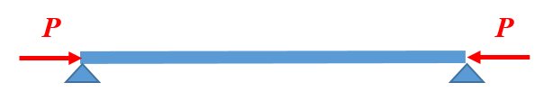
A rudakból épített acélszerkezetek (pl. rácsos tartók) egyik jellegzetes alkotó eleme a nyomott rúd. Nyomott rúdról akkor beszélünk, ha a rendszerint egyenes tengelyű szerkezeti elem központos P nyomóerővel terhelt (1. ábra).
A 2. ábra a nyomott rúd méretezésének fejlődését illusztrálja. Kezdetben (a régi időkben) az építőmesterek az évszázadok során felhalmozódott tapasztalati ismeretek alapján, amelyek mesterről tanítványra szálltak, állapították meg a különböző anyagú és méretű nyomott oszlopok teherbírását. Jelentős változást a klasszikus matematikai differenciálanalízis mérnöki alkalmazása hozott. Euler (1707-1783) svájci matematikus és fizikus megoldotta a nyomott rugalmas vonal kihajlásának problémáját, amely megoldás alkalmazható volt a rugalmas nyomott rúd megoldására (Euler erő). A mérnökök a következő évszázadokban felismerték, hogy az Euler erő csak bizonyos esetekben (elsősorban nagy karcsúságoknál) ad elfogadható közelítést a nyomott rúd valós teherbírására. Számos, az Euler képletnél fejlettebb megoldás született a nyomott rúd teherbírására, de jelentős változást csak a II. világháborút követő hatalmas szerkezetépítési konjunktúra hozott. A világ minden számottevő szerkezeti laboratóriumában sorra végezték a nyomott rúd kísérleteket, majd az eredményekből összeállítottak egy több mint kétezer kísérletből álló adatbázist. A nyomott rúd teherbírását az adatbázis alapján, a matematikai statisztika módszerével meghatározott képlettel adták meg.
Ez a módszertan a mai napig meghatározó: „a nyomott rúd méretezése az acélszerkezeti szakma politikai kérdése lett…”. Ezért a nyomott rúd méretezési elvének megértése a szerkezet-építőmérnök számára alapvető fontosságú.
Az ábra jobb oldala a jövőre is tartalmaz utalást. A tudományos kutatás szintjén már jelen, hogy a valós nyomott rúd teherbírását matematikai-mechanikai szimulációval is meg lehet határozni. Sőt, a közeljövőben minden eddigi ismeretet meghaladó adatbázisok hozhatók létre a szuperszámítógépek bevetésével. Egy ilyen gigantikus adatbázis alapján a mesterséges intelligencia felülírhatja az eddigi mérnöki tudást és módszertant, legalábbis elvben. A valóság viszont az, hogy a szerkezet-éptőmérnökség nem tartozik a húzóágazatok közé (mint például a hadipar vagy az autóipar), ezért ez az új méretezéselméleti váltás még egy jó ideig bizonyosan várat magára.

A továbbiakban a ma acélszerkezeti mérnöksége számra kiemelten fontos Euler erőt és a kísérleti alapú szabványos méretezési formulát tárgyaljuk részletesen.
Az ideális nyomott rúd teherbírása: az Euler erő
Tételezzük fel, hogy az alábbi ábrán látható csuklósan megtámasztott nyomott rúd rendelkezik az alábbi tulajdonságokkal:
- tökéletesen egyenes,
- az anyaga tökéletesen lineárisan rugalmas,
- központosan nyomott.
A fenti feltételekkel végezzük el a nyomott rúd kísérletet a Consteel szoftver segítségével: futtassuk a lineáris kihajlási analízis (Linear Buckling Analysis, LBA) számítást. Az eredményt a 3. ábra szemlélteti.
gateA Consteelben a 3. és 4. osztályú szelvények keresztmetszeti interakciós ellenállása az EN 1993-1-1 6.2 képlet módosított változatával kerül kiszámításra, az öblösödés és a komponens ellenállások előjelhelyes figyelembevételével. Lássuk, hogyan…
GATEDid you know that you could use Consteel to determine the optimum number of shear connectors for composite beams?
In composite beam design, the required number of shear studs is not only a detailing issue but a direct part of the structural resistance mechanism. The modelling and design environment in Consteel allows this number to be determined in a rational and automated way, consistent with EN 1994-1-1:2010.
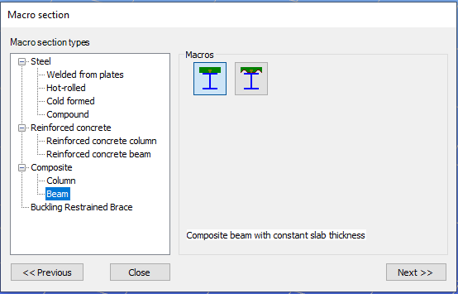
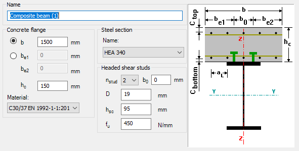
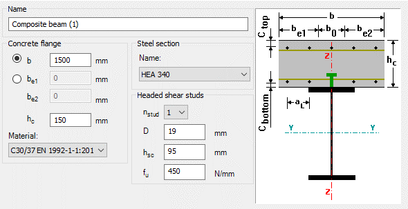
The process begins with the definition of a composite beam cross-section (Macro section). Two standard types are available: a solid slab composite beam and a profiled steel sheeting composite beam. The effective width is defined at input level, but the actual effective width used in analysis is calculated automatically based on span, geometry, and stud spacing assumptions. This ensures that the structural response is captured realistically, while maintaining simple input control for the user.
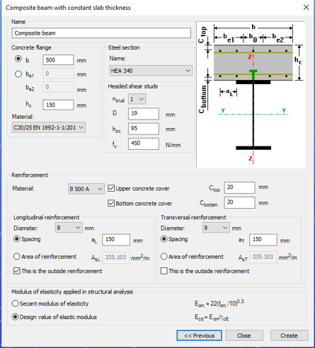
After defining the cross-section, the member is created and design parameters are assigned through object properties. These parameters govern key aspects of composite behaviour, including stud spacing, support conditions, and whether shear stud design is performed manually or automatically.
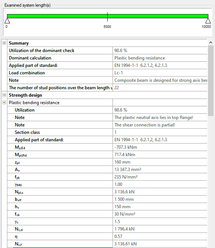
For shear connector design, Consteel applies a plastic distribution model. The governing section of the beam, typically corresponding to the maximum bending moment, is identified automatically. From this section, shear studs are distributed symmetrically along the beam length.
When automatic optimisation is selected, the software determines the minimum number of shear studs required to satisfy bending resistance. It then increases the number iteratively until the composite section achieves sufficient capacity. The resulting value represents the optimal number of shear connector positions for the given loading and geometry.

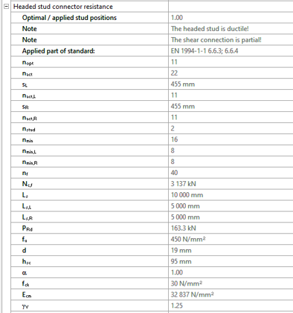
The key parameters used in this evaluation include:
- nopt: optimal number of shear stud positions in the governing region
- nact: actual number of stud positions applied
- sL, sR: spacing of studs on the left and right side of the critical section
- nmin: minimum required number of stud positions based on resistance
The ratio nact / nopt is used as a direct measure of utilisation of the shear connector system.
There is also the option to define the number of studs manually. In that case, Consteel distributes them uniformly along the member and checks compliance with detailing rules such as minimum and maximum spacing. This is typically useful when construction constraints or predefined detailing standards take priority.
Composite beam design itself is carried out according to EN 1994-1-1:2010. Plastic bending resistance is evaluated for Class 1 and 2 cross-sections, while shear, concrete flange crushing, and longitudinal shear are checked at critical sections. Shear buckling is treated according to EN 1993-1-5. Lateral-torsional buckling is not included in the current design scope.
For profiled sheeting, shear stud resistance is reduced depending on rib orientation, in line with Eurocode 4 rules.
Overall, the key point is that the number of shear connectors is no longer an assumed input. It is derived from structural demand through an automated and transparent process, which makes it easier to reach an efficient and consistent composite design without repeated manual iteration.
Download the example model and try it!
Download modelIf you haven’t tried Consteel yet, request a trial for free!
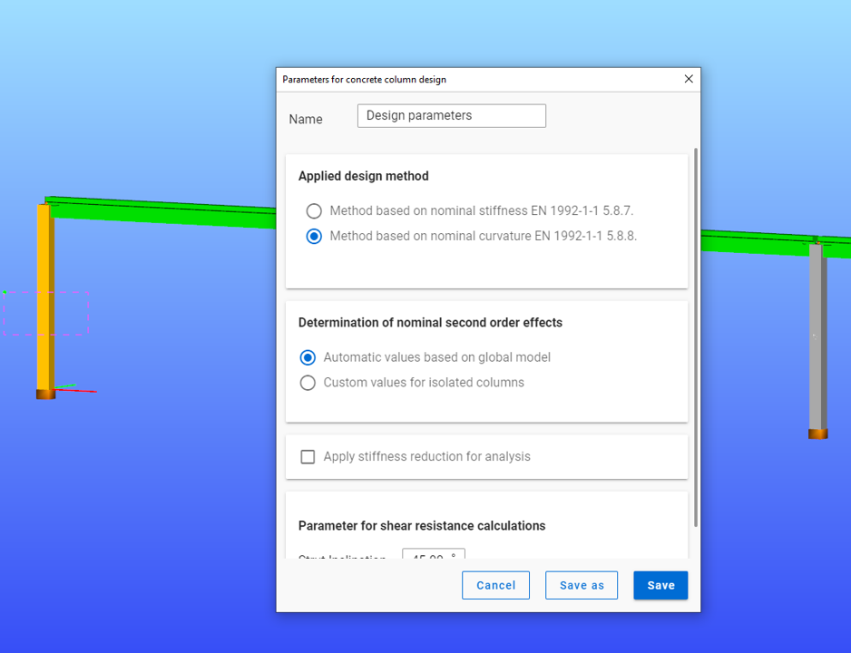
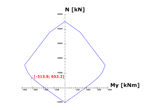
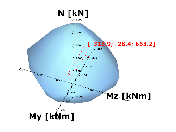
Try Consteel for freeDid you know that you could use Consteel to determine automatically the second order moment effects for slender reinforced concrete columns?
Download the example model and try it!
Download modelIf you haven’t tried Consteel yet, request a trial for free!
Try Consteel for free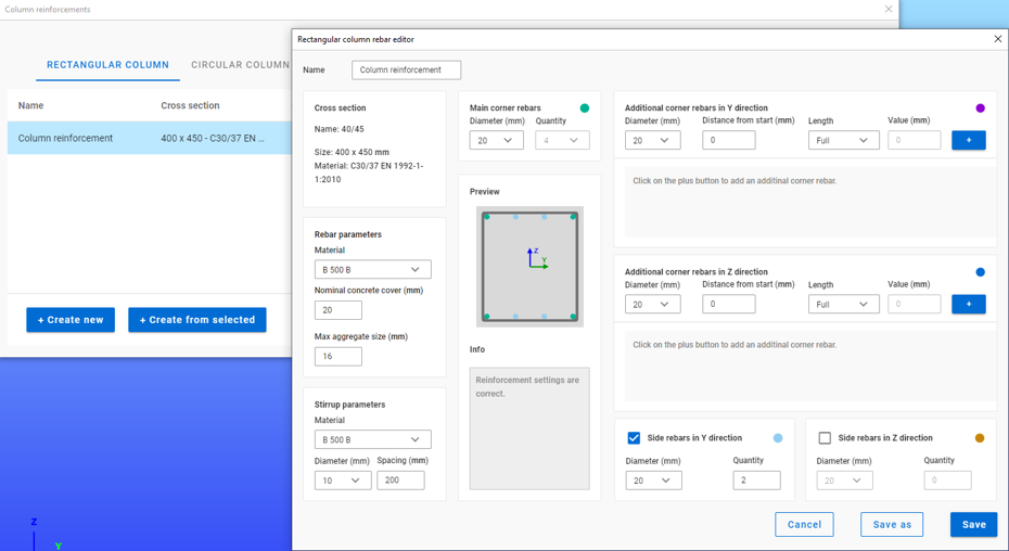
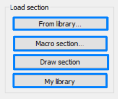
Did you know that you could use Consteel to perform local and distortional buckling checks for cold-formed members?
First, sections must be loaded into the model. To load cold-formed sections, you can choose from four options: From library, Macro section, Draw section, or My library.
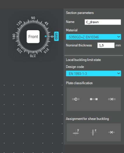
After the first-order and buckling analyses are completed, you can proceed to the Ultimate limit state check settings and enable the steel design cross-section and buckling checks. At the bottom of the steel design section, there is an option to Consider the supplementary rules from EN 1993-1-3 for the design of cold-formed sections. This checkbox must be selected if you want to design cold-formed sections.
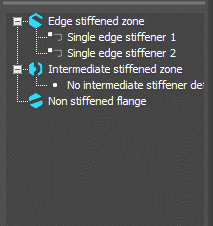
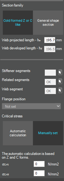
When the calculation is finished, by opening the Section module, we can review all the properties of the Effective section of the elastic plate segment model. By opening each plate element, we can verify the length, effective length, thickness, effective thickness, slenderness, and reduction factor separately. In addition, the properties of the stiffeners can also be verified: area, moment of inertia, lateral spring stiffness, critical stress, reduction factor, compressive stress, reduced effective area, and reduced thickness.
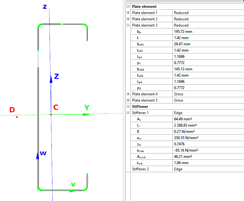
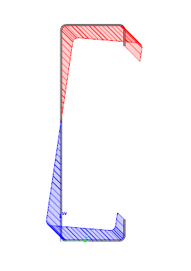
Similarly, the stresses can also be checked from the Properties tab. In the colored figure or diagram view, all the calculated stresses can be seen together with their resultants.
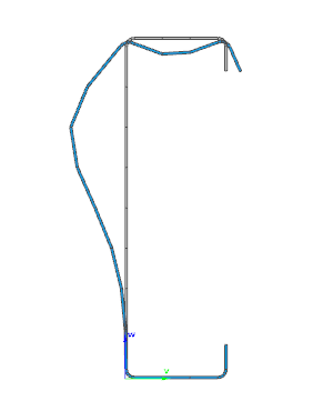
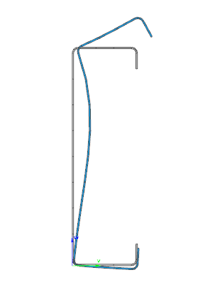
Consteel automatically takes into account the effect of distortional buckling when calculating the effective sections of cold-formed thin-walled sections.
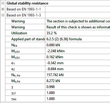
Moving on to the Standard resistance tab in the Section module, all calculated results can be verified, not only the dominant one. By opening the Global stability resistance check, we can see that, since we enabled the option to consider the supplementary rules from EN 1993-1-3 for the design of cold-formed sections, results are available both according to EN 1993-1-1 and according to EN 1993-1-3.
Download the example model and try it!
Download modelIf you haven’t tried Consteel yet, request a trial for free!
Try Consteel for free