Software version: ConSteel 17 Build 3303
Keywords: Modeling; Analysis; Design; Lattice girder; Getting started;
Model examples
Design objective, choice of design standard
This design guide is intended for novice ConSteel 17 users and provides a step-by-step guide for designing a simply supported lattice girder. The geometry of the lattice girder to be designed is known from the architectural conceptual design, (Figure 1). According to the concept, the lattice girder chords are made of hot-rolled sections of HEA120, while the lattice bars are made of cold-formed SHS80x4 sections. The design of the connections is not included in this guide.

(based on conceptual design)
It is well known that structural design is always carried out according to a certain standard or its version. The selection of the standard can be made from the Design Standard menu when creating a new model in the Project Center, or it can be modified later in the Standards tab [S1] selection panel (Figure 2).
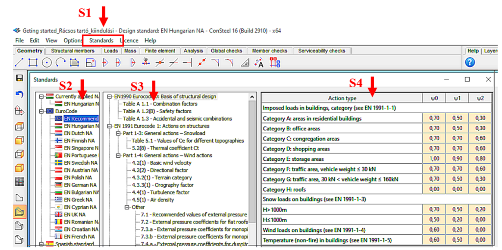
(S1: access standards; S2: select applicable standard; S3: select standard content; S4: display standard parameters).
The desired design standard can be selected from the list on the left of the panel. In this case, we select the EN Recommended option [S2]. The parameters applied by the selected standard can be accessed by selecting the corresponding row of the middle table [S3] of contents in the right-hand table [S4]. In Figure 2, the combination factors corresponding to Table 1.1 of the EC0 standard have been selected, whose parameters are shown in the right-hand table.
Setting the grid raster editor
First, let’s set the size of the raster according to the span of the structure by using the corresponding button [1] of the tool group on the left, which will bring up the Grid and Coordinate System adjustment panel (Figure 3).
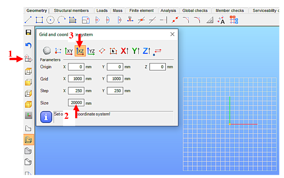
(1: set raster grid and coordinate system; 2: set raster occupancy size; 3: select view)
For example, for the 19.6m long support, the Size window can be set to 20000 millimeters [2]. To update the setting, press Enter. With the above setting, the raster will be 20m wide in X and Y directions, the raster line density will be 1000mm, and the step spacing will be 250mm. It is convenient to add the grid support model in the X-Z global coordinate plane, so the raster editor will be rotated to the X-Z plane. To do this, select the XZ plane option [3].
Loading initial cross-sections
One fundamental characteristic of general structural analysis programs is that they can only work with specifically defined cross-sections. Therefore, the first step is to choose the initial cross-sections for the task, according to the conceptual design. This may seem contradictory to the simple manual methods taught in basic statics courses, where the specific dimensions of the cross-section were often irrelevant information (e.g. calculation of internal forces). When using computer programs, however, we need to provide specific cross-sections even if their dimensions do not affect the static quantities to be calculated (e.g. in the present case, the normal forces of a truss beam). Nevertheless, we should aim to select cross-sections that match the geometrical size of the structure. In this case, the preliminary design served this purpose.
Initially, the section library for the current model is empty, so we first need to select the appropriate cross-sections. To do this, go to the Structure Members tab [4] and select the Section Administration option [5] on the left side of the horizontally positioned tool group, then select the “From Library…” button [6] in the panel that appears (Figure 4).

(4: picking up structural elements; 5: calling up the section control panel;
6: Select section type)
Figure 5 shows the loading of the HEA120 section, compliant with the European standard, which will be assigned to the chords. We select the region of the cross-section standard (European) and then its type (H profiles). From the list that appears, we can select the type of section (HEA) [7] and then the height of the section (120) [8]. By pressing the Load button [9], the program learns the cross-section, and from then on it knows everything about the cross-section and can work with it. Repeat the procedure as many times as you need different sections. Finally, the window is closed by pressing the Close button [10].
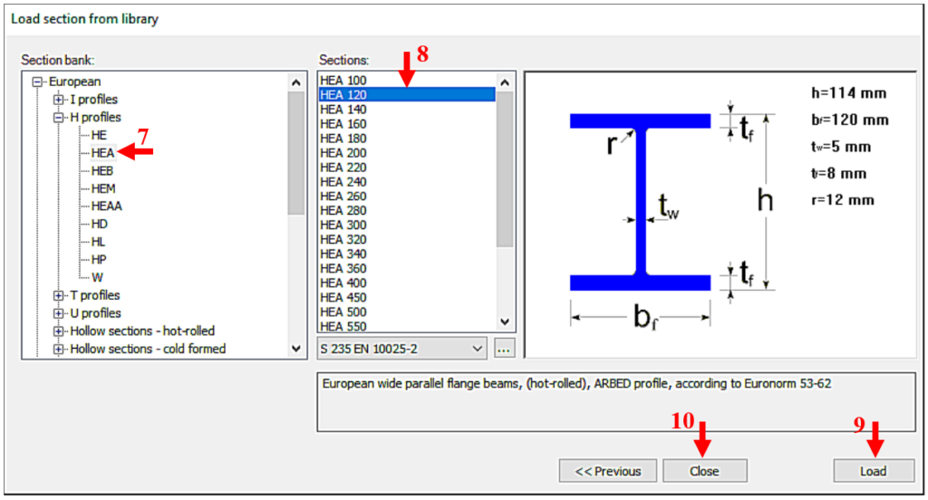
(7: select section type; 8: select section size; 9: scan selected section; 10: end loading process)
In our case, also a CF-SHS 80×4 closed section (from Library/Hollow sections – cold formed/CF-SHS/CF-SHS 80×4) was loaded for the bracing members (Figure 6).

Later on, you can obtain all the information about the cross-section using the Section module. To do this, select the cross-section in the table by clicking on the corresponding row and then click on Properties… to display all the properties of the cross-section, such as type data; cross-section characteristics, etc. The program works with two cross-section mechanical models in a dual manner. The GSS (General Solid Section) model [11] is used for static calculations and the EPS (Elastic Plate Segment) model [12] for standard design operations (Figure 7). The cross-sectional properties (surface area, moments of inertia, etc.) can be displayed by pressing the button [13].
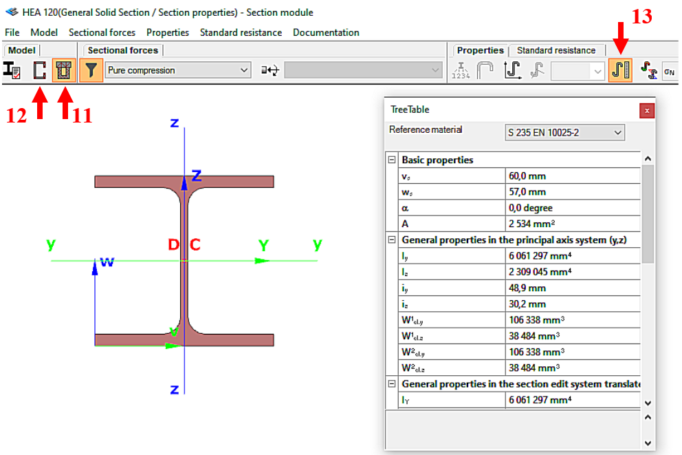
(11: Open GSS general section model; 12: Open EPS elastic plate segment model;
13: open cross-sectional properties table)
Designing a lattice girder
The design of the bars of a truss (lattice girder) structure does not require any special theoretical knowledge: normally, the truss bars are designed as compressed and/or tensioned bars, neglecting bending moments and shear forces. The dimensioning of compression bars is nowadays carried out using a model-based computer procedure. For details, see the knowledge base material Design of columns against buckling. Here, only the determination of the deflection length of the compressed bars is presented.
The most important parameter for the dimensioning of a compressed bar is the slenderness:
$$\overline{\lambda}=\sqrt\frac{Af_y}{N_{cr}}$$
where
$$N_{cr}=\frac{\pi^2El}{(kL)^2}$$
where the buckling length factor k is recommended by EN1993-1-1 to facilitate manual calculations:
| Type of the bar | Direction of buckling | k |
|---|---|---|
| chord | – in-plane – out-of-plane | 0.9 0.9 |
| bracing | – in-plane – out-of-plane | 0.9 1.0 |
Software using model-based computational methods (e.g. Consteel software) determines the elastic critical force Ncr directly by finite element numerical methods, taking into account the behaviour of the entire lattice girder, instead of the above conservative formula. The following example is intended to illustrate the relationship between the manual design procedure proposed by the standard and the results of the modern model-based numerical procedure.
- Let the structural model of the lattice girder under consideration be the Consteel model shown in Figure 1.
- Let the load shown correspond to the design load combination of the girder.
- Determine the deflection length of the most stressed compressed chord member using finite element numerical stability analysis.
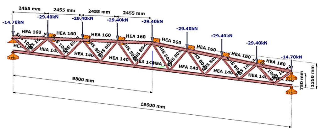
(Consteel software)
Relationship between procedures
The steps of the calculation are:
Buckling stability analysis
The stability analysis of the elastic model shows the governing buckling mode of the lattice structure and the corresponding elastic critical load factor αcr (Figure 2).
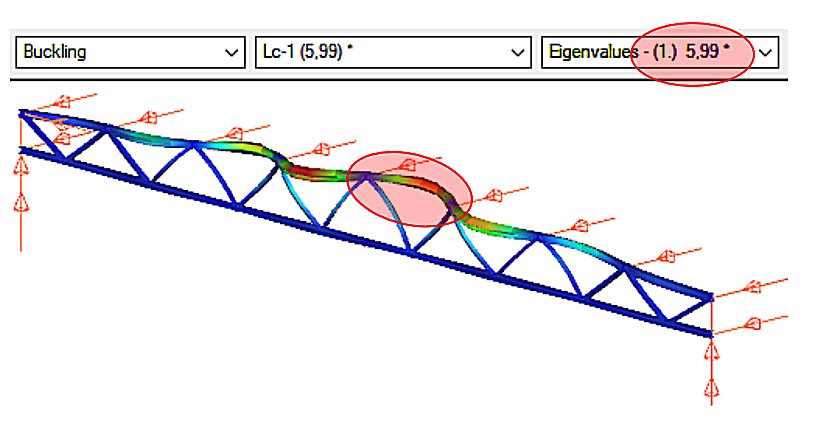
We can see that the upper chord of the perfectly elastic model is deflected laterally under load. The load that causes this elastic buckling is the critical load, whose value is given by the product of the design load and the critical load factor αcr=5.99.
gateThe evolution of compressed bar (column) design
One of the characteristic features of steel structures made of bars (e.g. lattice girders) is the compressed bar. We speak of a compressed bar when the structural element, which usually has a straight axis, is loaded by a compressive force P applied centrally (Figure 1).

Figure 2 illustrates the evolution of compressed bar (column) design. In the beginning (in the old days), master builders determined the load-bearing capacity of compressed columns of different materials and sizes on the basis of the experience accumulated over the centuries, passed down from master to apprentice. A significant change was brought about by the application of classical mathematical differential analysis to engineering. The Swiss mathematician and physicist Euler (1707-1783) solved the problem of the deflection of a compressed elastic line, which could be applied to the solution of the elastic compressed bar (Euler’s force). In the following centuries, engineers recognised that Euler’s force only gave an acceptable approximation to the real load capacity of a compressed bar in certain cases (mainly for large slender bars). Many solutions for the bearing capacity of a compressed bar were developed that were more advanced than the Euler formula, but it was not until the huge structural engineering boom following World War II that significant changes were made. Compression bar experiments were carried out in every major structural laboratory in the world, and a database of over two thousand experiments was compiled from the results. The load capacity of the pressure bar was given by a formula based on the database, using the method of mathematical statistics.
This methodology is still dominant today: ‘the dimensioning of the compressed bar has become a political issue for the steel construction profession…’. Understanding the principle of compressed bar design is therefore essential for the structural engineer.
The right side of the Figure 2 also contains a hint for the future. At the level of scientific research, it is already present that the load capacity of a real compressed column can be determined by mathematical-mechanical simulation. Indeed, in the near future, databases that go beyond anything we know today can be created using supercomputers. On the basis of such a gigantic database, artificial intelligence could, at least in principle, supersede existing engineering knowledge and methodology. But the reality is that structural engineering is not one of the pull sectors (such as the defense or automotive industries), so this new shift in design theory is certainly a long way off.
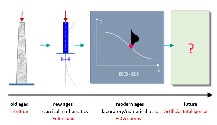
In the following, the Euler force and the experimentally based standard design formula, which are of major importance to structural steel engineering today, are discussed in detail.
Buckling strength of the ideal columns: the Euler force
Assume that the hinged compressed column shown in the Figure 3 has the following properties:
- perfectly straight,
- its material is perfectly linearly elastic,
- centrally compressed.
Under the above conditions, perform the compressed column experiment using Consteel software: run the Linear Buckling Analysis (LBA) calculation. The result is illustrated in Figure 3.
gateThe latest version, Consteel 17 is officially out! In 2023, our main focus for Consteel development is improving usability. New features prioritize efficient model manipulation, easy modification, and clear information presentation across Consteel, Descript, and our cloud-based platform, Steelspace. In this comprehensive video, we walk you through a step-by-step workflow guide, demonstrating how to leverage Consteel 17 to its full potential.
If you would like to delve deeper into the new features, check out our detailed blog post for an in-depth exploration of Consteel 17’s capabilities.
Did you know that you can use Consteel to design simple supported, continuous and over-lapped purlins systems in Consteel, considering shear and rotational stiffness of attached roof sheeting?
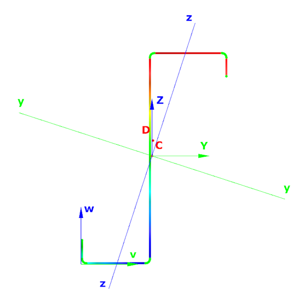
To use the purlin design functions, you first need to place cold formed Z or C purlins in your model, these are the only profile types supported for purlin design. All functions related to purlin lines can be found in the Structural members tab.

With these three main functions you can define the purlin line object, specify the support zones, and set the overlap zones. A detailed explanation of each can be found in the Consteel Manual – Purlins Chapter.
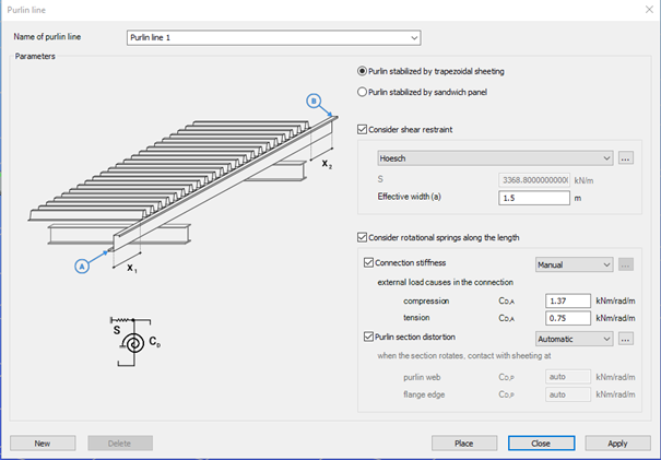
The Place purlin line function allows you to create and configure a purlin line object and place it precisely within your structural model.
You can also control the sheeting eccentricity in the Z direction, either by selecting predefined positions or by entering custom values. A graphical interface supports these settings to ensure intuitive and accurate placement.
An important feature of this function is the ability to simulate the supporting effect of roof sheeting on the purlins. This is done by applying spring stiffnesses that reflect how the sheeting contributes to the overall structural behavior. Two types of springs are considered:
- Translational (shear) spring, representing the shear stiffness of the roof covering.
- Rotational spring, accounting for both the connection stiffness and profile distortion.
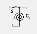
Depending on the selected sheeting type (trapezoidal sheeting or sandwich panels) the stiffness values can be entered manually or calculated automatically. Automatic calculations follow the guidelines of EN 1993-1-3, providing reliable and standards-based results.
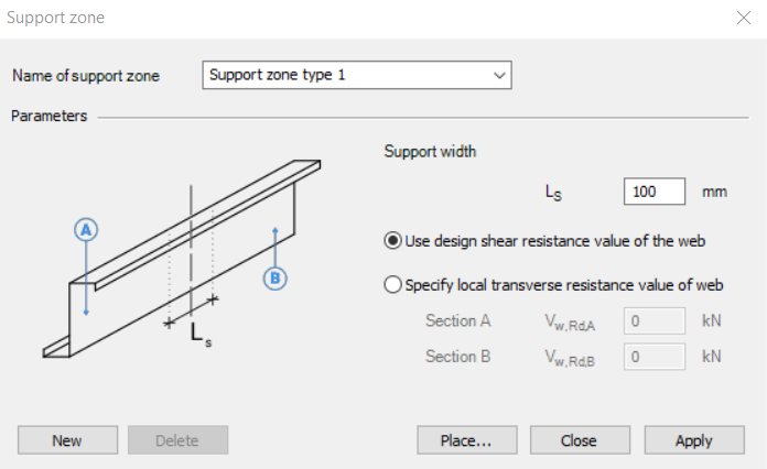
The Support zone function allows you to define the geometrical and mechanical parameters at the points where the purlins are supported. The geometry and bearing capacity can be set by specifying the support width and selecting how the load capacity is defined.
The Purlin overlap function helps define how individual purlins are connected in continuity. The standard (EN 1993-1-3) distinguishes between simple overlap joints and joints with coupling elements. Currently, only overlap joint is available in the program. You can define the length of the overlap either in millimeters or as a percentage of the member length. Additionally, the stiffness distribution between the two overlapping members can be adjusted.
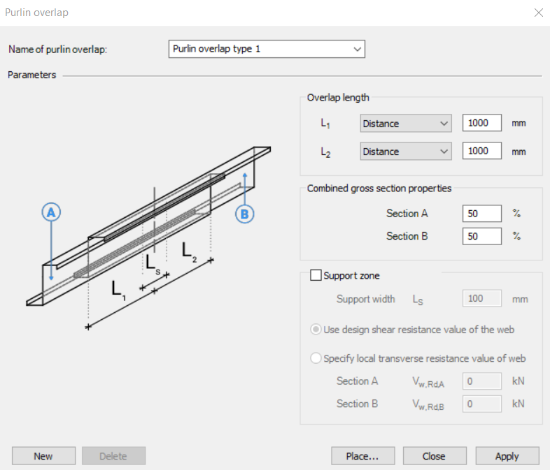
Together, these functions ensure accurate modeling of purlin behavior, support conditions, and connection details, aligning with design standards and practical requirements.
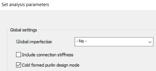
To ensure that all purlin line related objects are properly considered in the analysis, make sure to activate the Cold formed purlin design mode in the analysis settings. When this mode is enabled, both the buckling analysis and the global design are performed on a submodel that includes only those members associated with purlin line objects. This mode is intended exclusively for the design of the roof purlin system.
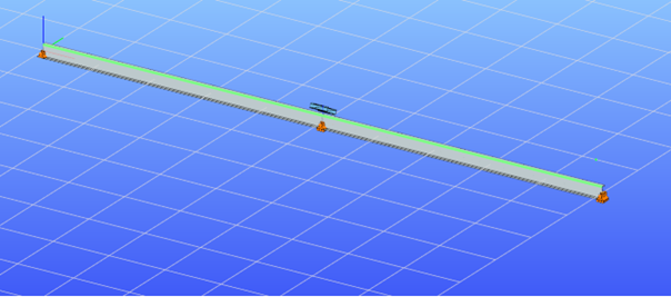
If purlin related objects are present in the model but the cold formed purlin design mode is not active, the structural elements connected to these objects will be excluded from the second-order stiffness matrix. As a result, their influence will not be considered during linear buckling or second-order analysis.
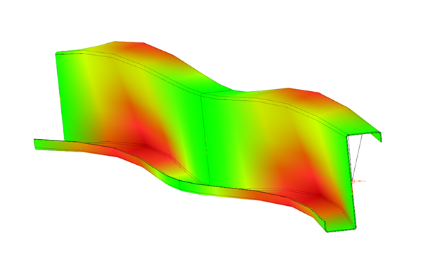
Download the example model and try it!
Download modelIf you haven’t tried Consteel yet, request a trial for free!
Try Consteel for freeIn Consteel, the calculation of cross sectional interaction resistance for Class 3 and 4 sections is executed with the modified Formula 6.2 of EN 1993-1-1 with the consideration of warping and altering signs of component resistances. Let’s see how…
Application of EN 1993-1-1 formula 6.2
For calculation of the resistance of a cross section subjected to combination of internal forces and bending moments, EN 1993-1-1 allows the usage -as a conservative approximation- a linear summation of the utilization ratios for each stress resultant, specified in formula 6.2.
$$\frac{N_{Ed}}{N_{Rd}}+\frac{M_{y,Ed}}{M_{y,Rd}}+\frac{M_{z,Ed}}{M_{z,Rd}}\leq 1$$
As Consteel uses the 7DOF finite element and so it is capable of calulcating bimoment, an extended form of the formula is used for interaction resistance calculation to consider the additional effect.
$$\frac{N_{Ed}}{N_{Rd}}+\frac{M_{y,Ed}}{M_{y,Rd}}+\frac{M_{z,Ed}}{M_{z,Rd}}+\frac{B_{Ed}}{B_{Rd}}\leq 1$$
Formula 6.2 ignores the fact that not every component results the highest stress at the same critical point of the cross-section.
In order to moderate this conservatism of the formula, Consteel applies a modified method for class 3 and 4 sections. Instead of calculating the maximal ratio for every force component using the minimal section moduli (W), Consteel finds the most critical point of the cross-section first (based on the sum of different normal stress components) and calculates the component ratios using the W values determined for this critical point. Summation is done with considering the sign of the stresses caused by the components corresponding to the sign of the dominant stress in the critical point.
(For class 1 and 2 sections, the complex plastic stress distribution cannot be determined by the software. The Formula 6.2 is used with the extension of bimoments to calculate interaction resistance, but no modification with altering signs is applied)
Example
Let’s see an example for better explanation.
GATEDid you know that you could use Consteel to design web-tapered members?
Tapered members are widely used in the economic design of steel-framed structures, such as industrial halls and warehouses, because they make it possible to save material while still ensuring structural strength and stability. With Consteel’s dedicated Tapered Member function, you can model, analyze, and verify these members efficiently, supporting both everyday engineering practice and advanced stability checks.
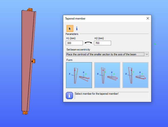
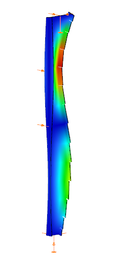
In Consteel, tapered members are line members with welded I or H, box, or cold-formed C sections. Hot-rolled and other macro sections cannot be tapered. Their section height can vary linearly along the member length, making them suitable for realistic structural modeling.
It is best to start with a section close to the smaller end of the taper. The start height (H1) applies at the beginning of the member, and the end height (H2) at the other end. If either value is less than half of the original section height, Consteel automatically resets it to 0.5 times the original. H1 and H2 can be swapped easily with the dedicated icon to reverse the taper direction.
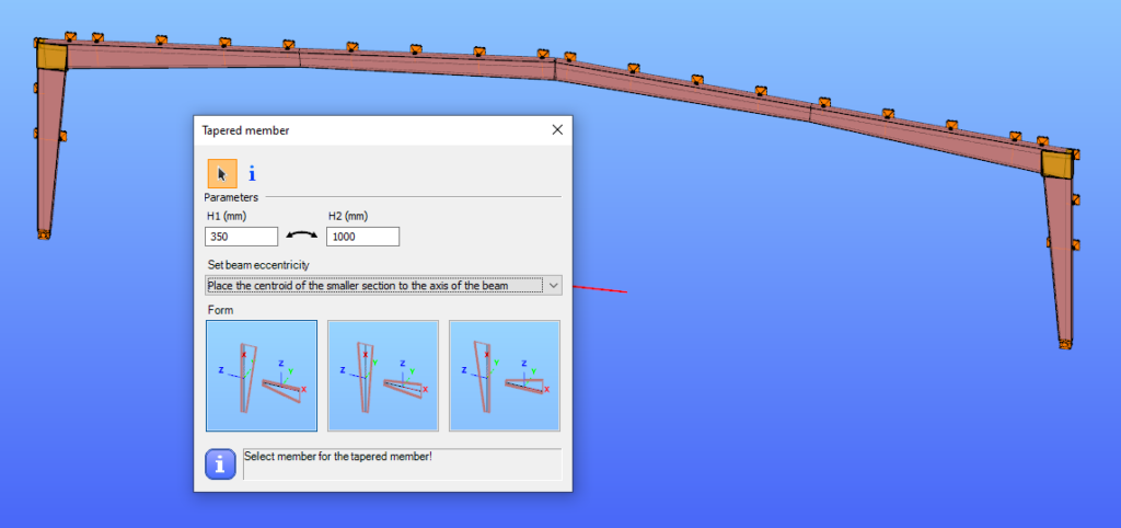
The placement of a tapered member relative to the axis of the original beam is defined by beam eccentricity rules. Consteel offers three alignment options:
- Centroid of the smaller section on the axis – the tapering develops outward from the end with the smaller height.
- Centroid of the larger section on the axis – the bigger end of the member remains fixed to the original axis.
- Centroid of the original section on the axis – one edge of the tapered member coincides with the original section, and the tapering starts from this position.
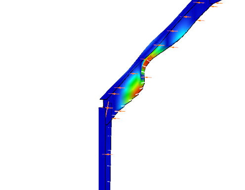
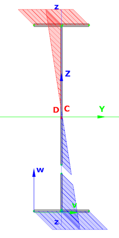
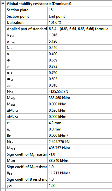
In analysis, Consteel creates tapered sections with the specified start and end heights and places them on the member’s reference line. Unless symmetric tapering is used, this placement is eccentric, which introduces additional effects. At frame joints, for example, extra moments from eccentric axial forces must be considered to maintain equilibrium.
Consteel handles these effects automatically, ensuring realistic results. Symmetric tapering keeps the analysis simpler, while eccentric tapering requires more attention. In all cases, global stability checks should complement sectional verifications to guarantee structural safety.
Download the example model and try it!
Download modelIf you haven’t tried Consteel yet, request a trial for free!
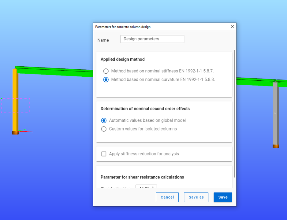
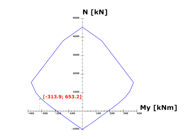
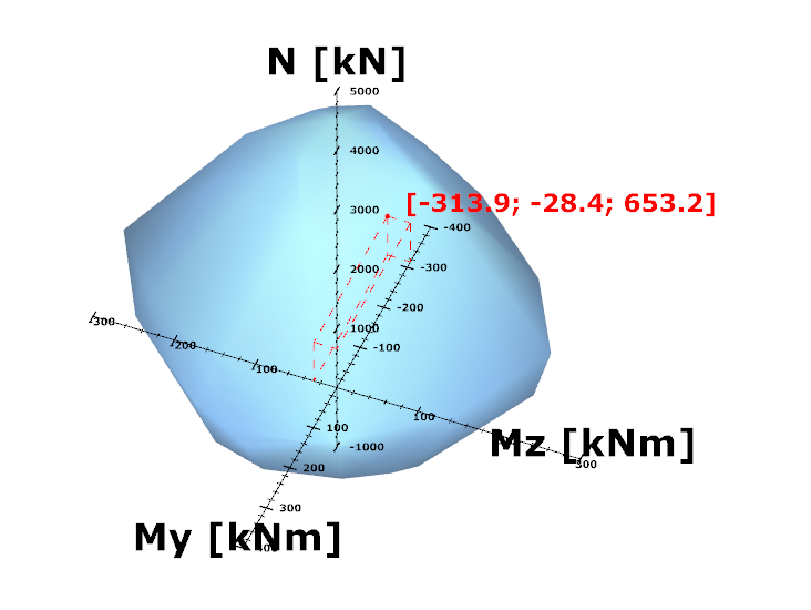
Try Consteel for freeDid you know that you could use Consteel to determine automatically the second order moment effects for slender reinforced concrete columns?
Download the example model and try it!
Download modelIf you haven’t tried Consteel yet, request a trial for free!
Try Consteel for free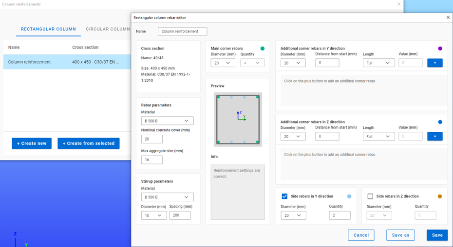
Did you know that you could use Consteel to perform local and distortional buckling checks for cold-formed members?
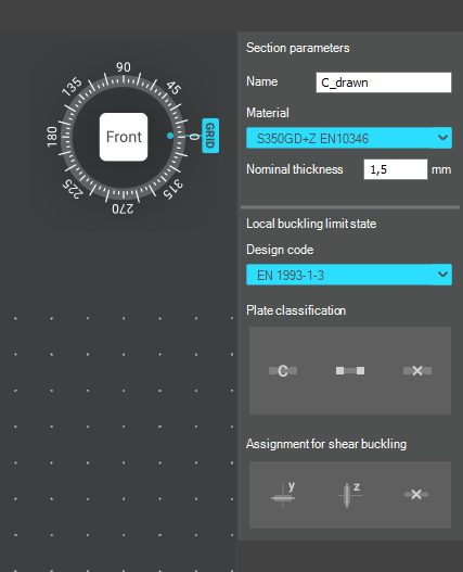
First, sections must be loaded into the model. To load cold-formed sections, you can choose from four options: From library, Macro section, Draw section, or My library.

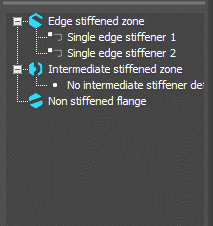
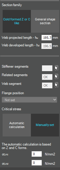
After the first-order and buckling analyses are completed, you can proceed to the Ultimate limit state check settings and enable the steel design cross-section and buckling checks. At the bottom of the steel design section, there is an option to Consider the supplementary rules from EN 1993-1-3 for the design of cold-formed sections. This checkbox must be selected if you want to design cold-formed sections.
When the calculation is finished, by opening the Section module, we can review all the properties of the Effective section of the elastic plate segment model. By opening each plate element, we can verify the length, effective length, thickness, effective thickness, slenderness, and reduction factor separately. In addition, the properties of the stiffeners can also be verified: area, moment of inertia, lateral spring stiffness, critical stress, reduction factor, compressive stress, reduced effective area, and reduced thickness.
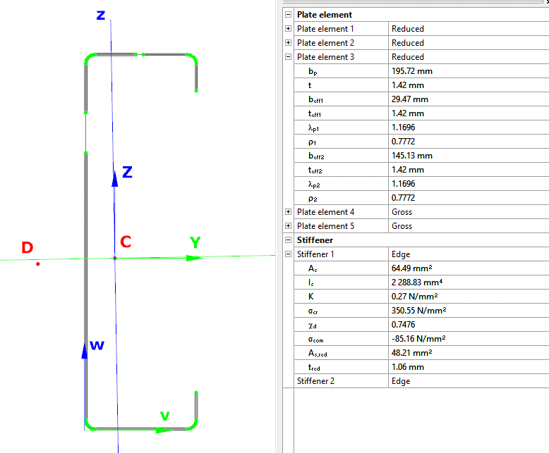
Similarly, the stresses can also be checked from the Properties tab. In the colored figure or diagram view, all the calculated stresses can be seen together with their resultants.
Consteel automatically takes into account the effect of distortional buckling when calculating the effective sections of cold-formed thin-walled sections.
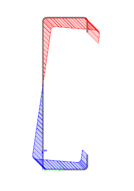
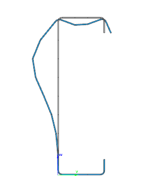
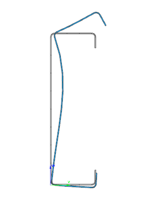
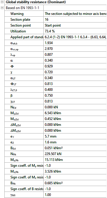
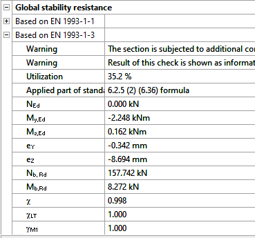
Moving on to the Standard resistance tab in the Section module, all calculated results can be verified, not only the dominant one. By opening the Global stability resistance check, we can see that, since we enabled the option to consider the supplementary rules from EN 1993-1-3 for the design of cold-formed sections, results are available both according to EN 1993-1-1 and according to EN 1993-1-3.
Download the example model and try it!
Download modelIf you haven’t tried Consteel yet, request a trial for free!
Try Consteel for freeIntroduction
Reinforced concrete columns are essential structural elements in the construction industry. They are used, for example, in frame buildings, halls, family houses and bridges. They are used in both monolithic and prefabricated versions.
The designer aims to design safe and economical structures. As technology evolves, so do our building materials, and higher strength concrete can be produced at lower cost. As a result, the use of smaller cross-sections of columns can be advantageous.
As the columns become slenderer, stability issues and the calculation of second-order effects become more important. The ConSteel finite element program specializes in steel structures and therefore has fast and well automated solutions to stability problems.
Taking advantage of the existing features of the software, a new method for designing reinforced concrete columns, improved by ConSteel, has been made available in ConSteel version 16. It is based on the Nominal Curvature method described in Eurocode 5.8.8 [1].
To apply the Nominal Curvature Method, a lot of information is required, various material and geometric parameters. The purpose of this article is to show that the Nominal Curvature Method, as extended in ConSteel 16, answers all the questions that arise during design and is free of many of the shortcomings of the original method.
Overview of Eurocode 2 – desinging reinforced concrete columns
In this chapter, the design of reinforced concrete columns based on Eurocode 2, nominal curvature method, is presented in outline, focusing on the most important aspects.
Material parameters
Partial safety factors:
- Modulus of elasticity of concrete
?cE = 1.20 - Concrete
?c = 1.50 - Steel reinforcement
?s = 1.15
The material properties of concrete are dealt with in Eurocode 1992-1-1, Chapter 3.1.
Modulus of elasticity:
- Design value
- ?cd = ?cm/γcE
- Reducing the mean value with γcE partial safety factor
- Applicable in ULS
- In the case where creep is not considered, or considered elsewhere
- ?cd = ?cm/γcE
Creep
The calculation of the creep coefficient is discussed in EN 1992-1-1, chapter 3.1.4. Here, various factors are used to determine the final value of the creep coefficient as a function of concrete strength, using diagrams. The values can also be determined according to Annex B of EN 1992-1-1. The two calculations give almost identical results.
Imperfections
The imperfections of concrete buildings are discussed in Eurocode 1992-1-1, Chapter 5.2. It divides the imperfections into two parts. One is the global inclination, which is shown in Figure 1(b). The other part is when the network points are not displaced but the elements in between are curved. This is the initial curvature (also known as a shape error), illustrated in part c) of Figure 1.

Inclination
The effect of imperfection due to inclination can be taken into account by calculating fictitious transverse forces (nominal loads). To do this, the value of the applied inclination is calculated as follows:
- Base value of inclination
θ0 = 1/200 - Height-dependent reduction factor
αh = 2/√?
where ? is the height - reduction factor depending on the number of structural elements
αm = √0.5(1 + 1/?)
?: number of vertical structural elements bearing the total load - applied inclination
θi = θ0αhαm
Then, as shown in Figure 2, the ? the normal forces can be used to calculate the notional loads in the unbraced case: ?i = θi?.
In braced case, for example a hinged-hinged column, ?i force is not defined at the top of the column, but at the center, with the value: ?i = 2θi?.
![Isolated member with eccentric axial force or lateral force. Unbraced (left) and braced (right) - EN 1992-1-1 Figure 5.1(a) [1]](https://www.consteelsoftware.com/wp-content/uploads/2023/06/2_isolated-member-with-eccentric-axial-force-or-lateral-force.png)
Second order effects
The method described in EN 1992-1-1, chapter 5.8.8, is applicable by default to isolated columns with constant cross-section and normal forces.
The design method uses the maximum second-order moment (?2). Its distribution along the length is not directly determined. For the sake of simplicity and to be conservative, it is usual to assume this second order bending moment to be uniform along the length, but the standard also permits a sinusoidal or parabolic distribution.
If we can realistically determine the distribution of curvature, the Eurocode allows the use of the method for global structures (EN 1992-1-1 5.8.5 (3)), but this is not usually possible for manual methods due to the interactions between the elements.
To use this method, it is essential to specify the buckling length, the value of the second order bending moment depends on it. For this purpose, the standard allows the use of the factors used in the elastic theory (for cantilever ?0 = 2?, fix bottom – top hinged case ?0 = 0.7?, etc.).
Calculation of design bending moment:
?Ed = ?0Ed + ?2
where
?0Ed is the 1st order moment, including the effect of imperfections
?2 is the nominal 2nd order moment (including the effect of any curvature)
Calculation of second order bending moment from curvature
Determine the nominal curvature first:
1/? = ?r?φ1/?0
where
- ?r is a correction factor depending on axial load
- ?φ is a factor for taking account of creep
- 1/?0 is the theoretical (physical) curvature associated with failure
1/?0 = ε??/0,45?
The curvature belongs to the point where the concrete reaches its ultimate compressive strength ( ) and the tensioned reinforcement is starting to yield, i.e. the so-called “balanced” case.
The position on the design line is taken into account by the correction factor depending on axial load:
?r = (?u − ?)/(?u − ?bal)
where
- ? = ?Ed / Ac?cd
relative axial force
- ?Ed
design value of axial force
- ?Ed
- ?u=1+ω
- ω = As?yd / Ac?cd
mechanical reinforcement ratio - As
is the total area of reinforcement - Ac
is the area of concrete cross-section
- ω = As?yd / Ac?cd
- ?bal =0.4
value of n at maximum bending - (0.4 applicable in the absence of further information)
Factor for taking account of creep:
?φ = 1 + βφef ≥ 1
where
- φef = φ(∞,0) ?0Eqp / ?0Ed
effective creep
- ?0Eqp first order quasi-permanent bending moment (SLS)
- ?0Ed first order bending moment (ULS) – design combination
- ?0Eqp first order quasi-permanent bending moment (SLS)
- β=0,35 + ?ck/200−λ/150
- λ = ?0 / ?
slenderness - ?0
buckling length - i = √?c/?c
inertia radius of uncracked concrete
- λ = ?0 / ?
Second order bending moment
?2=?Ed?2
where
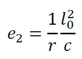
Second order eccentricity, where c is the factor depending on the curvature distribution. For constant cross-section ?=?2 applicable (sinusoidal distribution). In case of constant distribution ?=8 is applicable.
Design
Column Interaction Curve
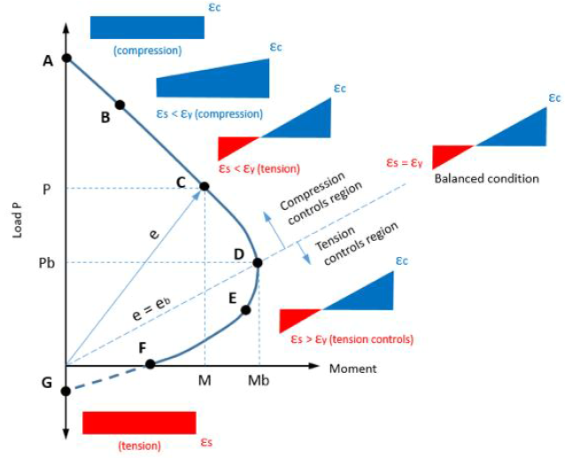
According to the Interaction Curve, the failure of the cross-section always occurs, when the concrete reaches its ultimate strain (usually ?cd = 0,35%).
Depending on where we are on the interaction curve, the reinforcement on the other side:
- Tensioned, and yielding,
- Tensioned, and just started yielding,
- Tensioned, but elastic,
- Compressed and elastic.
Theoretical background of the development
The design procedure is an extension of the standard procedure described in Chapter 2. It automates the manual entry of the buckling lengths and defines the distribution of the second order bending moments.
The initial value of the curvature distribution on which the calculation is based is performed on the global structure and not on an isolated column. The curvature distribution is determined from the elastic buckling shapes calculated on the whole structure (Linear Buckling Analysis – LBA).
This can be considered a realistic curvature distribution for the concrete column because we calculate the buckling shape for the entire structure, taking into account the interaction of the structural elements.
This allows the method to be extended, so that the column can now be considered not only as an isolated element, but also as part of the whole structure, in accordance with the Eurocode (EN 1992-1-1 5.8.5 (3)).
The final step, the calculation of second order bending moments (?2), is performed on an isolated model in the spirit of the standard, but for this curvature it uses the values of the corresponding buckling shape along the column calculated on the full model.
The maximum value of the buckling shape for the curvature prescribed by the standard (1/?) and the other values are varied in proportion.
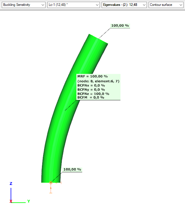
The appropriate eigenvalue assignment is done by a procedure called buckling sensitivity analysis. Magnification is performed at the point of maximum curvature found along the length of the column.
With this method, we could theoretically calculate second-order moments for any structural element and the entire structure. However, at this stage of development, it is only considered for straight-axis beam elements defined as reinforced concrete columns.
Later on, if the need arises, the procedure can be developed into a general procedure after proper testing and verification. This could be a very useful feature for example for reinforced concrete arches or reinforced concrete frame columns with moment restraints.
Buckling sensitivity analysis
The main difficulty of the method is to find the right buckling shapes for the corresponding RC columns ins both direction (x and y). The program calculates a number of buckling shapes defined by the user.
Assuming each shape as a displaced shape, the summed deformation energy per bar element is calculated along each bar element of the structure.
The element with the highest deformation energy value calculated on the basis of the buckling length just tested is assigned a value of 100%, the other elements a proportional value. The buckling shape currently under consideration is assigned to the corresponding bar element.
Since a column can generally bend in both perpendicular directions, the test is performed in both local directions and 2 eigenvalues are assigned to each column (1-1 per direction).
Calculation of second order bending moments
According to Eurocode:
?2 = ?Ed?2

where ? = π2
ConSteel calculates in a similar manner. Second order moments are calculated for each finite element of the reinforced concrete column. Three values are used. The first is the normal load at the finite element point (?Ed). The second is the second order eccentricity as defined in the Eurocode (?2).
After that, the third value is the ordinate of the buckling shape at the given finite element point, with the maximum of the buckling shape normalized to the unit value. Simply put, multiplying the first two values by this third value gives the second order moment at the given finite element point of the reinforced concrete column. This results in an improved moment distribution.
Differences compared to the standard procedure
Simplification of the calculation of the effective creep:
φef = φ(∞,?0)
conservatively, we equate the effective creep with the final value of the creep factor, without reduction. This avoids errors such as, for example, if there is no bending moment in a quasi-permanent load combination, then the value of the effective creep factor is by definition zero.
Creep factor value in ConSteel
The values given in ConSteel are taken from Table 1 of the Eurocode guide for Reinforced Concrete Structures [6].
This is based on EN 1992-1-1, chapter 3.1.4, where various factors can be used to determine the final value of the creep factor as a function of concrete strength, using diagrams.
Calculation of slenderness based on buckling analysis

Critical strength of the Euler beam. The formula rearranged:

where

There is no need to manually enter the buckling length, the slenderness calculation is fully automated.
Second order bending moment distribution
The distribution of the second order bending moment is the same as the buckling shape, taking into account the interaction between columns.
Demonstration of the method using a console example
You can see how to make the example model in our Reinforced Concrete Column – overview article.
Download the starter model at the end of this article and open the “separate_circle_column_cantilever.csm” file.
First order analysis
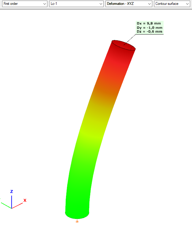
Displacement shape: realistic values:
- Slight vertical displacement
- in the direction where a greater horizontal load is applied, greater displacement
- slight displacement in the other direction due to the imperfection
- the displacement shape is curved in the direction of the horizontal load as expected
Check the internal forces:
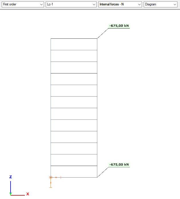
N
- same as the vertical load, with constant distribution (no self-weight applied in the model)
negative sign -> compression
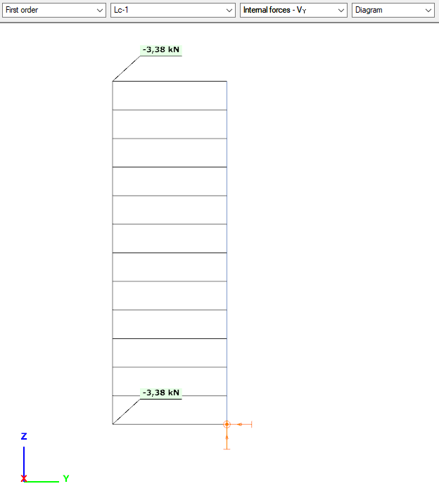
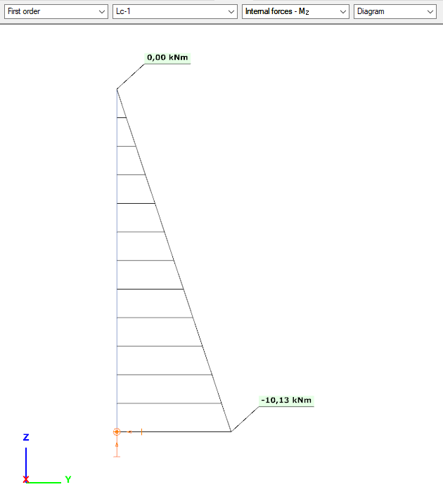
Vy+Mz
- we calculate the imperfection from the normal force
- 675*0,005 = 3,375 kN
- 3,38*3 = 10,14 kNm
- Distributions and valuer are as expected
- No Vy+Mz from applied loads, only from imperfection
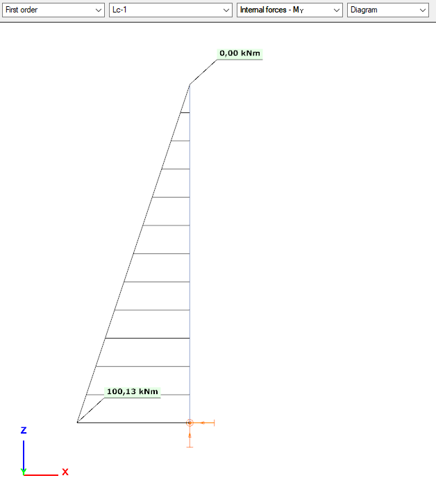
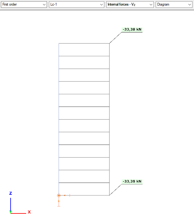
Vz +My
- Imperfection calculated form the normal force
- 675*0,005 = 3,375 kN
- 3,38*3 = 10,14 kNm
- These internal forces are calculated from imperfection
- Additional 20*1,5 = 30 kN load
- 30+3,375 = 33,375 kNm
- 33,375*3 = 100,125 kNm
- Correct internal forces
- first order internal loads from applied loads + inclination
Buckling analysis & buckling sensitivity analysis
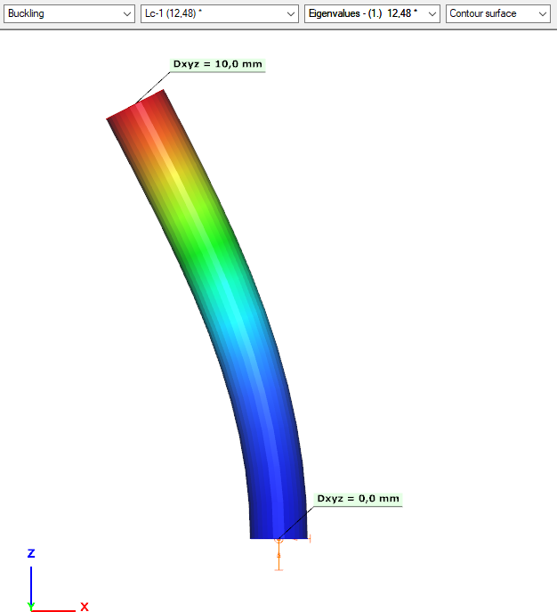
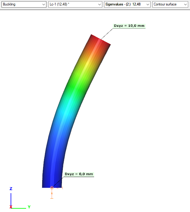
We can see from the coordinates, that this is indeed a planar buckling shape.
For a single column, it is rather easy, to check whether we have buckling shape in both directions. Here we only found one, so we need to find the other one as well.
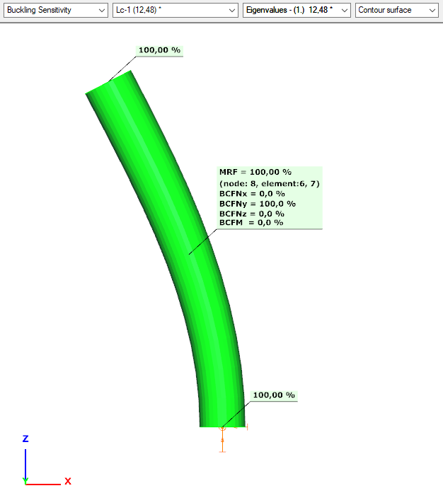
Parameters of the buckling analysis need to be adjusted. We should increase the upper limit of the calculated number of buckling shapes.
Download the adjusted model at the end of this article and open the “separate_circle_column_cantilever_MoreBucklingShape.csm” file.
Now we have buckling shape in both x and y directions.
ULS design – EN 1992 condition
Everything is symmetrical.
GATE
