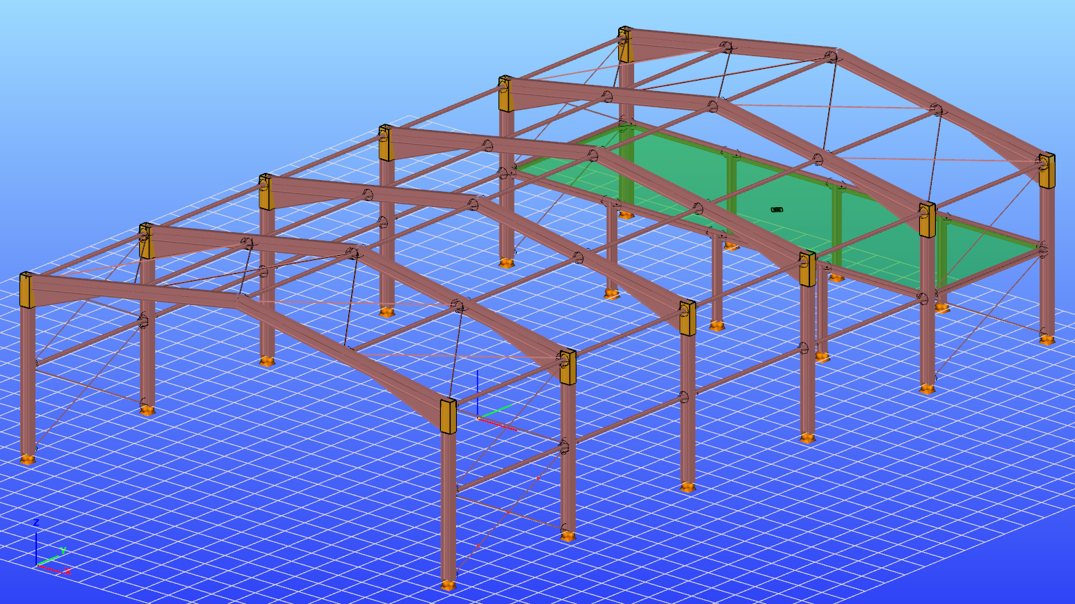
The practical use of the ‘General method’ of EN 1993-1-1 6.3.4 for the buckling design of global structural models is still a challenging issue requiring several problems to solve. In this paper we propose a fully developed methodology presenting solutions for the application topics such as the suitable FE model, specific modeling issues to capture the true 3D behavior of the members and the whole model and the final evaluation of the design parameters. The presented methodology consistently uses a unique model for the evaluation of all analysis and design parameters and results and yields a fully automatic design process controlled solely by the properly created structural model.
Click the button bellow to download and read the full article.
gateThe results of analyzes of frames with a span of 12, 15 and 18 m have been presented. Their minimum mass was assumed as the optimization criterion. The finite element method was used in the calculations. The results of calculations in the form of: structure mass, bar resistance coefficient and checking the SLS condition were presented in the tables.
Click the button bellow to download and read the magazine brochure. (PL)
gateWarehouse building example for Overall Imperfection Method in Consteel

Watch our user guide about How to use the Overall Imperfection Method to learn more.
gateOverall Imperfection Method in Consteel
The Overall Imperfection Method is an alternative way to carry out the buckling design for a structural member. With this method the buckling phenomenon is considered on the effect side of the equation, instead of on the resistance side, compared to the general method and the member check method. In the following video we explain the theoretical background for this calculation. After that we present application examples starting with the simplest ones, all the way to the most general case in a real-world building structure, showcasing the several extra capabilities and advantages of the Overall Imperfection Method.
Check out our user guide to learn more!
gateExample model for calculate critical temperature in Consteel
Watch our user guide about How to use the critical temperature feature to learn more.
gateCritical temperature calculation in Consteel
The calculation of the critical temperature is available in Consteel since the release of version 14. As an introduction of this feature, we prepared a video that gives some theoretical background on the topic, and demonstrates its usage in Consteel. It is shown how to prepare the model, how to execute the analysis and design, and how to create documentation about the critical temperature results.
Check out our user guide to learn more!
gateConsteel 14 is a powerful analysis and design software for structural engineers. Watch our video how to get started with Consteel.
Contents
- Build joint model based on the global model
- Bolted moment end-plate connection design
- Base plate connection design
- Apply connection stiffness in analysis
Consteel 14 is a powerful analysis and design software for structural engineers. Watch our video how to get started with Consteel.
Contents
- Set design parameters
- Perform cross section check
- Examine the design results in the Section Module
- Stability design according to the general method
- Member check – stability design for members
- Serviceability check
In our series we have shown in Part 1 and Part 2 how the spring stiffness „K” is determined for and edge and for an intermediate stiffener. In this part we will show how to proceed further.
The goal is to determine how efficiently can this stiffener support the connected compressed plate. To consider local buckling of the compressed plate the effective widths will be calculated. These widths can be either calculated for a plate supported at both ends or for a plate supported at one end only, using Table 4.1 and Table 4.2, respectively.
If a stiffener fulfills the minimum constructive requirements, we will first assume that it is rigid enough the act as a support. Based on this we work out the effective lengths for the connected compressed plates, assuming also that they are fully loaded up to the yield strength. Once we know the effective widths of the plate parts connected to the stiffener, we also know the load this stiffener is supposed to be able to carry without buckling, to justify the first assumption. Therefore, next we calculate the flexural buckling resistance of the stiffener. If we find out that it is lower than what was implicitly assumed previously, we go back to the first step, lower the stress to be compatible with the obtained buckling resistance of the stiffener (distortional buckling). This lower stress level may of course result different effective widths. An iterative procedure is started until the satisfactory result is found. After completion the final stiffener buckling resistance value will be incorporated into an equivalent effective thickness applicable for the stiffener and the connected effective plate parts.
In the above described iterative process the „K” value of the stiffener will be needed to determine the flexural buckling resistance of the stiffener. This resistance will be calculated using the help of a simple beam model, where the stabilization provided the remaining parts of the section is used as a continuous bedding of „K”. The cross section of the beam corresponds to the stiffener and connected plate parts and will be exposed to the actual stress level of the iteration, assumed as a simplification to be constant along the length. The length of the beam in this model is unknown at the moment, it should be equal to the half wavelength of the buckling shape which is expected to be around 1.5-3 times the height of the studied cold-formed section.
Distortional buckling will appear only if the length of the stiffener is much longer than this typical length range. As a further simplification Eurocode assumes infinite length as the possible worst case, because for this condition an analytic solution exists in the literature:

In this formula „K” is the spring value – shown in Part 1 and Part 2 – represents the spring stiffness value what the remaining section can provide to the stiffener. Isand Asare section properties of the corresponding stiffener together with connected effective widths of supported plates, namely area and inertia around an axis perpendicular to the expected direction of buckling of the stiffener. E is the Young modulus of the steel material.
The formula gives the critical stress level where elastic buckling would appear. Once this has been found, reduced slenderness is calculated, and the distortional buckling resistance can be obtained by using a special buckling curve given by (5.12a-c) formulas of EN 1993-1-3.
The validity of formula (5.15) can be easily demonstrated with a simple Consteel model.
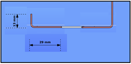
Let’s assume the Z section from our 1st blog exposed to compression force and let’s assume that we have already calculated effective width values. Yield strength of the material is 235 MPa and coating thickness is 0.04 mm. We found that the effective width of the lip and flange are ceff=13 mm and beff=29 mm, respectively.
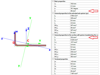
The section properties can be calculated with Consteel
Distortional buckling – Further secret formulas of EN 1993-1-3. Check our article for the first secret formula if you hadn’t read it yet.
In our series we continue with the second „secret” formula of EN 1993-1-3.

This formula (5.11) is used when the ability of an intermediate stiffener to stabilize a compressed web plate is studied.
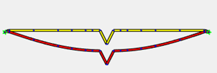
When the intermediate stiffener is rigid enough, it divides efficiently the longer web plate into shorter plates. During buckling a rigid stiffener will not displace and the plate will buckle between the ends (stabilized by flanges) and this stiffener:
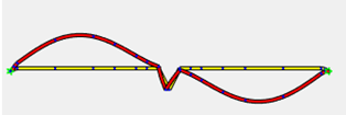
If the stiffener is not rigid enough, already at a much lower stress level the distortional buckling will appear which is characterized by a displacement of the stiffener and by the web plate buckling with a half-wave equal to the plate length:
In such a case Eurocode still accepts that web plate buckling will occur between ends and intermediate stiffener, but reduces the thickness of the intermediate stiffener zone, to compensate for the less than ideal rigidity. This compensation will depend on the buckling resistance of the stiffener when subject to compression.
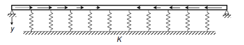
The simplified model used by Eurocode in the procedure can be seen below. As a simplification it is assumed that the web plate is connected to the rest of the section with hinges. It means that it’s buckling shape is not influenced by the stiffness of connected parts, they do not encaster its ends, its ends can freely rotate. The ends of the plate are supported and there the plate can provide an elastic bedding to the stiffener, which will be considered as a „help” when its buckling resistance will be determined. This bedding is represented by the K spring stiffness:
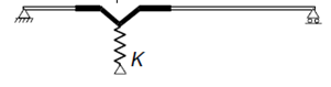
The spring value which represents in this model the bedding provided by the plate is calculated as the ratio of the displacement obtained from the application of a unit load at the center of gravity of the stiffneer. In this case the unit load is applied perpendicularly to the web plate. Formula (5.11) gives the deflection (δ) from such unit load (u).
gate